Project 2 - Rankine cycle Simulator
Aim:
To use Matlab to simulate a Rankine cycle.
Getting properties of steam and water from XSteam data (IAPWS IF - 97 standard)
User inputs are used to figure out all the state points of the cycle.
Drawing the T vs. s and H vs. s plots based on the data given.
Rankine Cycle:
The Rankine cycle is an idealised thermodynamic cycle or heat engine. It uses fuel to heat a boiler, which turns water into steam. The steam then expands through a turbine to make useful work. In 1859, a Scottish engineer named William J.m. Rankine came up with this method. It's a cycle that turns heat into mechanical energy, which is then usually turned into electricity. In this project, a cycle that fits the ideal is simulated. So, not counting losses.
The Rankine cycle is the ancestor of the Rankine cycle. The temperature differential between a heat source and a cold source determines how powerful it is. The greater the differential, the more effectively mechanical power can be converted from heat energy.
Since ideal cycles are merely theoretical, the efficiency of the Rankine cycle is constrained by friction losses, high heat of vaporisation of the working fluid, etc.
Due to its advantageous characteristics, including its availability, cheap cost, non-toxic, and unreactive chemistry, as well as its thermodynamic characteristics, water is often the fluid of choice. The pressure at the turbine outlet is reduced by condensing the working steam vapour to a liquid, and the energy used by the feed pump uses just 1% to 3% of the turbine's output power, increasing the cycle's efficiency. The advantage of this is negated by the low steam temperature permitted to the turbine.
Working:
In the Rankine cycle, there are four processes that can happen in any order:
Process 1-2: The turbine's isentropic expansion.
Process 2-3: Constant pressure The condenser gets rid of heat.
Process 3-4: The pump uses isentropic compression.
Process 4-1: Adding heat to the boiler at a constant pressure.
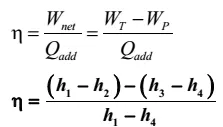
Rankine Cycle thermal efficiency:
BW ratio:
The amount of work done by the turbine that the compressor needs to do its job.
The BW ratio is Wp/Wt.
MATLAB Program:
clear all
close all
clc

disp(' RANKINE CYCLE ');
disp('1-2 is Constant pressure heat addition in the boiler');
disp('2-3 is Isentropic Expansion in the Turbine');
disp('3-4 is Constant pressure heat removal in the Condenser');
disp('4-1 is Isentropic compression in the pump');

p1 = input('nValue of pressure at turbine inlet, p1(in bar) = ');
T1 = input('nValue of temperature at turbine inlet, T1(in degree.C) = ');
p2 = input('nValue of pressure at condenser inlet, p2(in bar) = ');


% At State 1
h1 = XSteam('h_pT', p1, T1);        % Extracting Enthalpy at state pt 1
s1 = XSteam('s_pT', p1, T1);

% At State 2
s2 = s1;                            % Isentropic Expansion
sf2= XSteam('sL_p', p2);            % Saturated Liquid Entropy
sg2 = XSteam('sV_p', p2);           % Saturated Vapour Entropy
x2 = (s2-sf2)/(sg2-sf2);
hf2 = XSteam('hL_p', p2);
hg2 = XSteam('hV_p', p2);
h2 = hf2 + (x2*(hg2-hf2));

% At State 3
p3 = p2;                            % Constant pressure Heat rejection in Condenser
s3= XSteam('sL_p', p3);
h3 = XSteam('hL_p', p3);

% At State 4
s4 = s3;
p4 = p1;

% Work done by turbine
Wt = h1 - h2;

% Work done to run pump
v3 = XSteam('vL_p', p3);
Wp = v3*(p4 - p3)*100;
h4 = h3 + Wp;

%Net work
Wnet = Wt - Wp;

%Heat into the system
Qin = h1 - h4;

%Heat out of the system
Qout = h2 - h3;

%Thermal efficiency
thermal_eff = (Wnet/Qin)*100;

%Specific Steam Consumption
%SSC = mass flow rate/power
SSC = (3600/Wnet);

% Back Work ratio
BW = (Wp/Wt)


% Calculation of Temperatures at the state points
T3 = XSteam('Tsat_p', p3);
T2 = T3;
Cp4 = XSteam('Cp_ps', p4, s4);
Cv4 = XSteam('Cv_ps', p4, s4);
k = Cp4/Cv4;
T4 = T3/((p3/p4)^((k-1)/k));

%Calculating Temperature, Entropy and Enthalpy at the vapour and liquid line for plotting
T6 = XSteam('Tsat_p', p1);
s5 = XSteam('sL_p', p1);
s6 = XSteam('sV_p', p1);
h5 = XSteam('hL_p', p1);
h6 = XSteam('hV_p', p1);
T5 = T6;


%Plotting the saturation curve
T = linspace(1,375,1000);
for i = 1:length(T)

sf(i) = XSteam('sL_T', T(i));
sg(i) = XSteam('sV_T', T(i));
hf(i) = XSteam('hL_T', T(i));
hg(i) = XSteam('hV_T', T(i));
end

%Plotting T-s diagram
figure(1)
hold on
plot(sf, T, 'b','linewidth',2)
plot(sg, T, 'b','linewidth',2)
plot([s1 s2], [T1 T2], 'r', 'linewidth', 3)
plot([s2 s3], [T2 T3] ,'r', 'linewidth', 2)
plot([s3 s4], [T3 T4], 'r', 'linewidth', 3)
plot([s4 s5], [T4 T5], 'r', 'linewidth', 3)
plot([s5 s6], [T5 T6], 'r', 'linewidth', 3)
sc1 = linspace(s6, s1, 1000);
for l = 1:length(sc1)
 Tc1(l) = XSteam('T_ps', p1, sc1(l));
end
plot(sc1, Tc1, 'r', 'linewidth', 2)
text(s1+0.1, T1, '1')
text(s2+0.1, T2, '2')
text(s3, T3-20, '3')
text(s4, T4+20, '4')
title('Temp vs Entropy plot')
xlabel('Entropy ,S (Kj/kgk')
ylabel('Temperature (degree C) ')
legend('Saturation curve')


%Plotting h-s diagram
figure(2)
hold on
plot(sf, hf, 'k', 'linewidth', 1)
plot(sg, hg, 'k',  'linewidth', 1)
plot([s1 s2], [h1 h2], 'g', 'linewidth', 2)
plot([s2 s3], [h2 h3], 'g', 'linewidth', 2)
plot([s3 s4], [h3 h4], 'g', 'linewidth', 2)
hc = linspace(h4, h5, 100);
for r = 1:length(hc)
sch(r) = XSteam('s_ph', p1, hc(r));
end
plot(sch,hc, 'r', 'linewidth', 3)
plot([s5 s6], [h5 h6], 'b', 'linewidth', 3)
for m = 1:length(sc1)
hc1(m) = XSteam('h_ps', p1, sc1(m));
end
plot(sc1, hc1, 'g', 'linewidth', 3)
text(s1+0.1, h1, '1')
text(s2+0.1, h2, '2')
text(s3, h3-100, '3')
text(s4, h4 +200, '4')
title('Enthalpy vs Entropy plot')
xlabel('Entropy , S (KJ/kgk) ')
ylabel('Enthalpy , H (KJ/kg)')
legend('Saturation curve','location','northwest')


% Displaying the Results in the Command Window:
disp('Results');
p1 = p1;
T1 = T1;
p2 = p2;
disp('At stage point 1');
n1 = sprintf('P1 is %.3f bar',p1);
disp(n1);
n2 = sprintf('T1 is %.3f C',T1);
disp(n2);
n3 = sprintf('h1 is %.3f kJ/kg',h1);
disp(n3);
n4 = sprintf('s1 is %.3f kJ/kgK',s1);
disp(n4);
disp('At stage point 2');
n11 = sprintf('P2 is %.3f bar',p2);
disp(n11);
n21 = sprintf('T2 is %.3f C',T2);
disp(n21);
n31 = sprintf('h2 is %.3f kJ/kg',h2);
disp(n31);
n41 = sprintf('s2 is %.3f kJ/kgK',s2);
disp(n41);
disp('At stage point 3');
n12 = sprintf('P3 is %.3f bar',p3);
disp(n12);
n22 = sprintf('T3 is %.3f C',T3);
disp(n22);
n32 = sprintf('h3 is %.3f kJ/kg',h3);
disp(n32);
n42 = sprintf('s3 is %.3f kJ/kgK',s3);
disp(n42);
disp('At stage point 4');
n13 = sprintf('P4 is %.3f bar',p4);
disp(n13);
n23 = sprintf('T4 is %.3f C',T4);
disp(n23);
n33 = sprintf('h4 is %.3f kJ/kg',h4);
disp(n33);
n43 = sprintf('s4 is %.3f kJ/kgK',s4);
disp(n43);
n14 = sprintf('Wt is %.3f kJ/kg',Wt);
disp(n14);
n15 = sprintf('Wp is %.3f kJ/kg',Wp);
disp(n15);
n16 = sprintf('Wnet is %.3f kJ/kg',Wnet);
disp(n16);
n17 = sprintf('Thermal_efficiency is %.2f Percent',thermal_eff);
disp(n17);
n18 = sprintf('SSC is %.2f kg/kWh',SSC);
disp(n18);
n19 = sprintf('Back work ratio is %.3f ',BW);
disp(n19);
Explanation:
Xsteam data is used to extract the enthalpy and entropy of water and steam at certain pressures and temperatures for SAT liquid and SAT vapour states, among other situations.
Pressure (in bars) at state point 1 (the turbine intake), the temperature at the same place (degrees Celsius), and pressure at the condenser inlet must all be entered into the programme (point 2).
The application calculates all the Rankine cycle state points using these inlets and data from Xsteam.
The Xsteam data operates as follows: h1 = XSteam('h pT', p1, T1); it provides the water's enthalpy in bar and degC at the specified pressure and temperature.
We further locate state points and extract their data from XSteam as we extract the data using thermodynamic relationships, which are discussed after studying the Rankine cycle.
After analysing the plots of Rankine cycles and extracting data from an Xsteam file, Sf and sg are calculated, along with hf and hg, where f and g stand for saturated liquid and saturated vapour, respectively.
Using the normal thermodynamic relation, the network, work from the turbine, work from the pump, and heat in and heat out are determined.
The Rankine cycle's efficiency and specific steam consumption (s.s.c.) are determined using thermodynamic relationships and mentioned in programmes employing those relationships.
For plotting purposes, T, s, and h is removed at the liquid and vapour lines after the fourth point to account for the fluctuation you see in the plot.
For saturated liquid and saturated gas, the saturation curve is displayed in red in T-S, while in H-S, it is black.
Using the plot command and specifying all of the labels, linewidth, colours, and titles, a plot of T versus s and h vs s is generated from all the points acquired by the programme.
As the user's input for the aforementioned inputs varies, the plot also changes.
The sprint command is used to show results on the command window.
Result:
The command window's input, output screen, and the many state points and parameters are shown below.
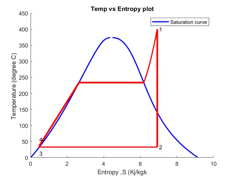
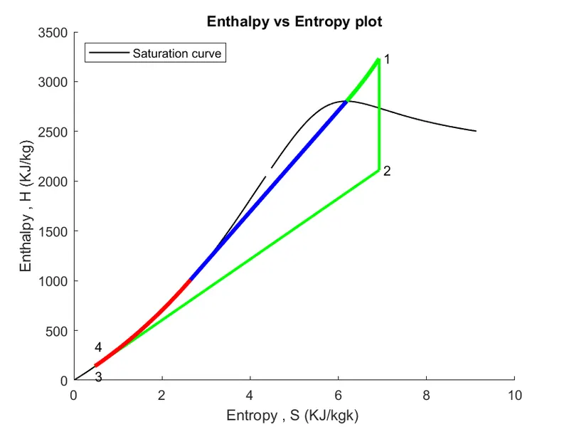
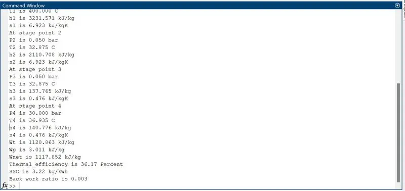
The net Work output is 1120.86 KJ/Kg.
The back work ratio is 0.003.
References:
https://skill-lync.com/challenges
https://imbooz.com/technical-articles/efficiency-of-rankine-cycle