Week 9 - FVM Literature Review

1.BASIC DEFENITION

a.Finite Difference method

The Finitie difference method converts the domain into set of dicrete points and a set of Partial Differential equations into a set of discrete equations called finite difference equations. The approximation of Derivatives is obtained using Taylor series.

b.Finite Volume method

The Finite Volume method divides the domain into small volumes. Governing equations are applied to each volume and simplified to obtain a set of algebraic equations.

1.DIFFERENCE BETWEEN FVM AND FDM

FDM

• Simple
• Difficult to apply to complex,3-D and curved geometires
• Efficient and easy to use for simple geometries
• Based on Differential form of Governing equations
• Easy to increase accuracy by going for a higher order of approximation
• Difficult to change the order of approximation or refinement locally -This causes problems in capturing discontinuties like stress concentration etc.

Applications-Weather Calculations, Astrophysics etc

FVM

• Can be aplied to complex,3-D and curved geometires
• Based on Integral form of Governing equations
• Local discontinuties can be better aprroximated by FVM as the local grid size can be easily changes however the order of fucntions that approximate the functions canot be easily changes as in FEM.This is a major disadvantage of FVM

Applications-CFD, Thermal problems, Chemical Engineering

2.NEED FOR INTERPOLATION SCHEMES

During approximation of surface and volume integrals we may require values other than the values at the computational nodes. In such cases Interpolation schemes are used

Examples of Interpolation schemes

2.(a) Upwind Interpolation scheme

The Upwind Interpolation or ‘donor cell’ Interpolation
scheme takes into account the flow direction when determining the value at a cell face.

For aproximating the value of a variable in the east face of a cell

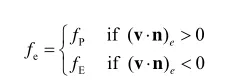
where fP and fE denotes the value at cell center of the cell west and east to the cell facerespectively

The scheme is first order accurate.

2.(b)Linear Interpolation scheme

The linear interpolation scheme uses linear interpolation to approximate the value at nodes other than computaional nodes. To estimate a value of a vairable at the cell face

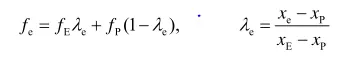
where fE and fP denotes the value at the cell center of the cells east and west to the Control voulme boundry respectively.

The scheme is equivalent to central differencing scheme and hence is second order accruate.

2.(c)Quadratic upwind interpolation (QUICK)

The upwind shceme is only first order accurate. It is prone to nuemrical diffusion.

Hence to counter this problem QUICK scheme was introduced

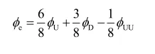
where D denotes downstream node and U denotes the first node upstream of the point whose value must be determined. UU denotes the second upstream node

The QUICK scheme is 3rd order sccurate but prone to oscilations

3.Need for Flux limitres

Lower order schemes like the Upwind method are first order accurate and introduce numerical dissipation. Higher order schemes like the QUICK method are prone to osillations. Hence our airm is to have a scheme which is higher order accurate but without oscillations.

Hence a class of schemes have been formulated to achieve oscilation free calculataions called TVD or Total Variation diminishing schemes.

What are TVD schemes

For a function to be stable,non-oscilatory and of higher order it has be monotonicity preserving. To be monotonicity preserving

1.It must not reate local maxima or minima

2.the value of a local maxima must be non-increasing and the value of a local minima must be non-decreasing.

Monotonicity decreasing schemes satisfy the property that the the total variatin of dicrete olution must diminish with time.Hence these scemes are called TVD

General representation of Upwind schemes

Upwind based schemes can be represnted as

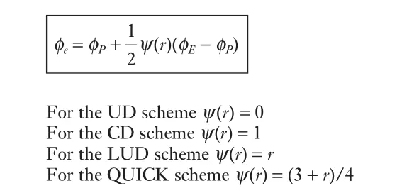
where

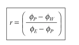
The ψ vs r diagram forms the basis for the scheme to be TDS

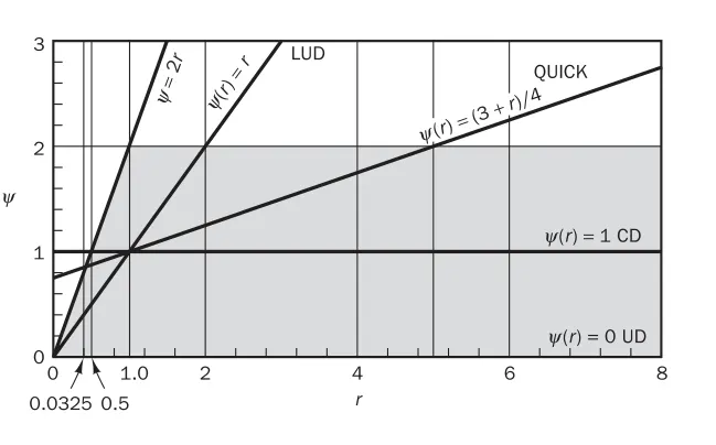
The Shaded area is where the schem is TDS

The idea of designing a TVD scheme is to introduce a modification to the above schemes so as to force the r–ψ relationship to remain within the shaded region for all possible values of r. This would imply that, in order to make the scheme TVD, we must constrain or limit the range of possible values of the additional convective flux ψ(r)(φE − φP)/2,which was originally introduced to make the scheme higher-order. Hence,the function ψ(r) is called a flux limiter function.

Hence Flux limiter fucntion is neccesary to ensure the scheme is TDS and hence stable , non-oscilatory and higher order.