Week 3 - Taylor table method and Matlab code

1.OBJECTIVE

To Derive the following 4th order approximations of the second-order derivative.

1. Central difference

2. Skewed right-sided difference

3. Skewed left-sided difference

for the function exp(x)*cos(x) and compare the solution obtained to the analytical derivative

2.Derivation of Nuemerical approximations

The derivation of Nuemerical approximations is done using Taylor's Table

For a skewed scheme the number of nodes(n) is given by

n=p+q

where p=order of derivative

q=order of approximation

therefore for the skewed schemes

n=4+2-1=5

2.(a) Central difference scheme

For a central scheme the number of nodes(n) required is given by

n=p+q-1

where p=order of derivative

q=order of approximation

therefore for the central difference scheme

n=4+2-1=5

Hence the nuemrical equation for approximation of second order derivative is

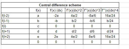
Solving the equations obtained using theabove Taylor table using OCTAVE to

A=[1 1 1 1 1; -2 -1 0 1 2 ;2 1/2 0 1/2 2;-4/3 -1/6 0 1/6 4/3; 16/24 1/24 0 1/24 16/24]
B=[0;0;1;0;0]
X=inv(A)*B

a=-0.083333
b=1.333333
c=-2.500000
d=1.333333
e=-0.083333

2.(b)Skewed right difference scheme

for a skewed scheme the number of nodes(n) required is given by

n=p+q

where p=order of derivative

q=order of approximation

therefore for the central difference scheme

n=4+2=6

Therefore a fourth order skewed right difference scheme

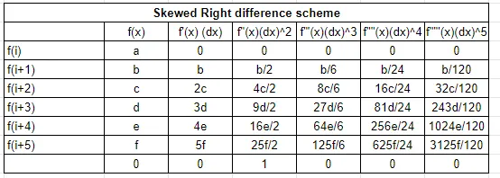
Solving the equations obtained using the above Taylor table using OCTAVE to

A1=[1 1 1 1 1 1; 0 1 2 3 4 5; 0 1/2 2 9/2 8 25/2;0 1/6 8/6 27/6 64/6 125/6;0 1/24 16/24 81/24 256/24 625/24;0 1/120 32/120 243/120 1024/120 3125/120]
B1=[0;0;1;0;0;0]
Y=inv(A1)*B1

a=3.75000
b=-12.83333
c=17.83333
d=-13.00000
e==5.08333
f=-0.83333

2.(c)Skewed Left difference scheme

The Taylor Table for skewed left difference shceme is as follows.

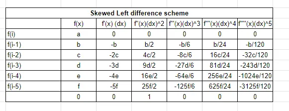
A2=[1 1 1 1 1 1; 0 (-1) (- 2) (- 3)  -4  -5; 0 1/2 2 9/2 8 25/2;0 -1/6 -8/6 -27/6 -64/6 -125/6;0 1/24 16/24 81/24 256/24 625/24;0 -1/120 -32/120 -243/120 -1024/120 -3125/120]
Z=inv(A2)*B1

a=3.75000
b=-12.83333
c=17.83333
d=-13.00000
e=5.08333
f=-0.83333

3.MAIN PROGRAM

clear all
close all
A=[1 1 1 1 1; -2 -1 0 1 2 ;2 1/2 0 1/2 2;-4/3 -1/6 0 1/6 4/3; 16/24 1/24 0 1/24 16/24];
B=[0;0;1;0;0];
P=inv(A)*B;
A1=[1 1 1 1 1 1; 0 1 2 3 4 5; 0 1/2 2 9/2 8 25/2;0 1/6 8/6 27/6 64/6 125/6;0 1/24 16/24 81/24 256/24 625/24;0 1/120 32/120 243/120 1024/120 3125/120];
B1=[0;0;1;0;0;0];
Q=inv(A1)*B1;
A2=[1 1 1 1 1 1; 0 (-1) (- 2) (- 3)  -4  -5; 0 1/2 2 9/2 8 25/2;0 -1/6 -8/6 -27/6 -64/6 -125/6;0 1/24 16/24 81/24 256/24 625/24;0 -1/120 -32/120 -243/120 -1024/120 -3125/120];
R=inv(A2)*B1;
x=pi/3;
dx=linspace(pi/4,pi/400,100);
f2=-2*exp(x)*(sin(x));
for i=1:length(dx)
Centraldifference(i)=(P(1)*expcos(x-2*dx(i))+P(2)*expcos(x-dx(i))+P(3)*expcos(x)+P(4)*expcos(x+dx(i))+P(5)*expcos(x+2*dx(i)))/(dx(i)^2);
skewedrightdifference(i)=(Q(1)*expcos(x)+Q(2)*expcos(x+dx(i))+Q(3)*expcos(x+2*dx(i))+Q(4)*expcos(x+3*dx(i))+Q(5)*expcos(x+4*dx(i))+Q(6)*expcos(x+5*dx(i)))/(dx(i)^2);
skewedleftdifference(i)=(R(1)*expcos(x)+R(2)*expcos(x-dx(i))+R(3)*expcos(x-2*dx(i))+R(4)*expcos(x-3*dx(i))+R(5)*expcos(x-4*dx(i))+R(6)*expcos(x-5*dx(i)))/(dx(i)^2);
Centraldifference_error(i)=abs(Centraldifference(i)-f2);
skewedrightdifference_error(i)=abs(skewedrightdifference(i)-f2);
skewedleftdifference_error(i)=abs(skewedleftdifference(i)-f2);
endfor
figure(1)
loglog(dx,Centraldifference_error,'b')
hold on
loglog(dx,skewedrightdifference_error,'r')
hold on
loglog(dx,skewedleftdifference_error,'g')
legend('Error-Central Differencing','Error-Skewed right differencing','Error-Skewed left differencing',"location","southeast")
title('Log Error vs log dx for various schemes')
xlabel('log(dx)')
ylabel('log(error)')
figure(2)
plot(dx,Centraldifference_error,'b')
hold on
plot(dx,skewedrightdifference_error,'r')
hold on
plot(dx,skewedleftdifference_error,'g')
legend('central differencing','skewedirght','skewedleft','analyticalderavative',"location","south")
xlabel('dx')
ylabel('Absolute value of error')
title('Absolute value of error vs dx')

4.FUNCTION

function y=expcos(x)
y=exp(x)*cos(x)
endfunction

5.RESULTS

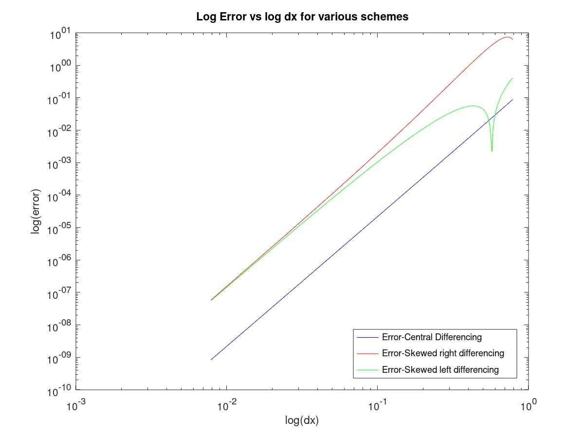
Skewed dfference schemes may be used if data from grid points is only availble from one side of the node.

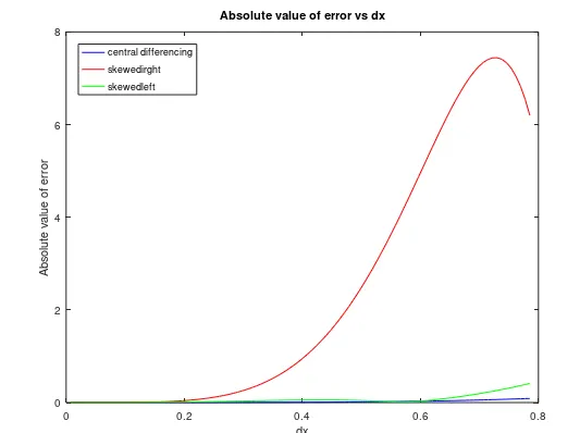
1.For all schemes as dx reduces i.e as the mesh becomes finer the error reduces. Giving more accurate results

2.The central difference scheme is more sccurate for almost all values of dx. In general the central difference scheme is more accurate than skewed scheme.

Why are skewed difference schems used?

Skewed dfference schemes may be used if data from grid points is only availble from one side of the node.