Week 7 - Simulation of a 1D Super-sonic nozzle flow simulation using Macormack Method
1.PROBLEM STATEMENT
To simulate flow in an isentropic quasi 1-D Convergent -Divergent nozzle using Mackmormack method.
The following results are to be obtained.
1.Steady-state distribution of primitive variables inside the nozzle
2.Time-wise variation of the primitive variables
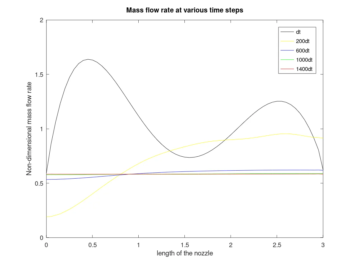
3.Variation of Mass flow rate distribution inside the nozzle at different time steps during the time-marching process
4.Comparison of Normalized mass flow rate distributions of both form
5.Conduct a grid indpedence test
2.THEORY
The below diagram gives the schematic of the problem
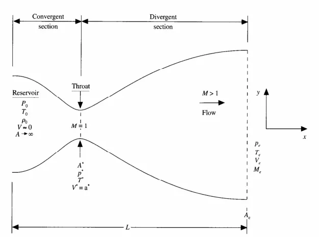
Fig-1:-Schematic of the problem. Source-Computational Fluid Dynamics by John D Anderson
The entry of the nozzle is connected to a reservior.Hence velocity at entry is nearly zero. The nozzle can be divided into 3 regions
1.Convergent part of the nozzle- Here the flow is subsonic i.e Mach number is less than 1
2.Throat- It is the section of the nozzle with minimum area. At the throat the flow is sonic
3.Divergent part of the nozzle- Here the flow is supersonic i.e Mach number is greater than 1
2(a).GOVERNING EQUATIONS
It is very common for flow feild variables to berepresented in non-dimensionalized form in case of nozzle flows. The same has been followed here
The Non Dimensionalized variables are as follows
Length
x'=x/L
where L denotes the length of the nozzle
Temperature
T'=T/T0
where T0 dentoes stagantion or reservoir temperature
Pressure
P'=P/P0
where P0 denotes stagnation or reservoir pressure
Density
ρ'=ρ/ρ0
where ρ0 denotes reservoir density
Velocity
v'=v/a0
a0 denotes speed of sound
Time
t'=t/L/a0
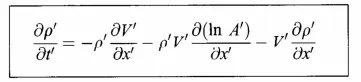
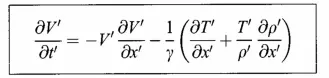
The Non-Dimensionalized Governing equations in Non-conservative form are
Continuity Equation
Momentum Equation
Energy Equation

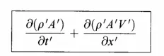
The Non-Dimensionalized Governing equations in Conservative form are
Continuity Equation
Momentum Equation
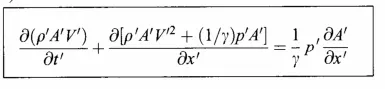
Energy Equation

The Conservative form of Governing equations can be conveniently represented inthe following form
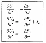
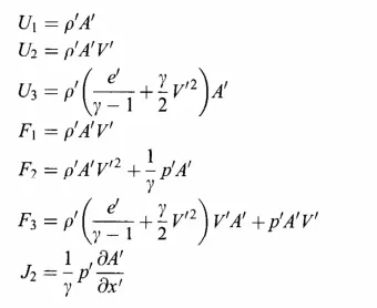
where
2.(b) Macormack method
The Macormack Method is a teachnique used to solve finite difference equations. It is second order accurate in time and space. The Macormack method is a predictor-corrector method.It consists of the following steps
1.The Predictor step:-In the predictor the spatial derivatives are discritized in forward difference. Provisional values of the variables are obtained
2.The Corrector step:-In the corrector step the spatial derivatives are discritized in backward difference.Values obtained using the predictor steps are used during substitution.
3.Average step:-The average of the time derivaitves obtained from predictor step and the corrector step is taken. This in turn is used to obtained values of flow variables for the next time step
3.PROGRAM
3.(a) MAIN PROGRAM
n=31;
y=1.4;
x=linspace(0,3,n);
dx=x(2)-x(1);
nt=1400;
C=0.5;
[Mfr_nc,rho_nc,T_nc,P_nc,M_nc]=Nonconserv(n,y,x,dx,nt,C);
[Mfr_c,rho_c,T_c,P_c,M_c]=Conserv(n,y,x,dx,nt,C);
figure(4)
plot(x,Mfr_nc,'g')
hold on
plot(x,Mfr_c,'b'))
xlabel('Lenght of nozzle')
ylabel('Non dimensional Mass flow rate')
legend('Nonconservative','conservative')
3.(b)FUNCTION FOR NON-CONSERVATIVE FORM
function [Mfr,rho,T,P,M]=Nonconserv(n,y,x,dx,nt,C);
%Initial profiles
rho=1-.3146*x;
a=1+2.2*(x-1.5).^2;
T=1-.2314*x;
v=(.1+1.09*x).*T.^0.5;
%Calculation of dt
for i=1:n
  dt1(i)=C*dx/((T(i)^(1/2))+v(i))
end
dt=(min(dt1))  ;
for i=1:nt
rho_old=rho;
T_old=T;
v_old=v  ;
%Predictor
for j=2:n-1
dvdx=(v(j+1)-v(j))/dx;
dTdx=(T(j+1)-T(j))/dx;
drhodx=(rho(j+1)-rho(j))/dx;
dlnadx=(log(a(j+1))-log(a(j)))/dx;
%Continuty Equation
drhodt(j)= -rho(j)*dvdx-rho(j)*v(j)*dlnadx-v(j)*drhodx;
%Momentum Equation
dvdt(j)=-(v(j))*(dvdx)-(1/y)*((dTdx)+((T(j)/rho(j))*drhodx));
%EnergyEquation
dTdt(j)=-v(j)*dTdx-(y-1)*T(j)*(dvdx+v(j)*dlnadx);
%Solution update
rho(j)=rho(j)+drhodt(j)*dt;
v(j)=v(j)+dvdt(j)*dt;
T(j)=T(j)+dTdt(j)*dt;
endfor
%Corrector
for j=2:n-1
dvdx_c=(v(j)-v(j-1))/dx;
dTdx_c=(T(j)-T(j-1))/dx;
drhodx_c=(rho(j)-rho(j-1))/dx;
dlnadx_c=(log(a(j))-log(a(j-1)))/dx;
%Continuty Equation
drhodt_c(j)= -rho(j)*dvdx_c-rho(j)*v(j)*dlnadx_c-v(j)*drhodx_c;
%Momentum Equation
dvdt_c(j)=-(v(j))*(dvdx_c)-(1/y)*((dTdx_c)+((T(j)/rho(j))*drhodx_c));
%EnergyEquation
dTdt_c(j)=-v(j)*dTdx_c-(y-1)*T(j)*(dvdx_c+v(j)*dlnadx_c);
endfor
%Average of derivative
  drhodt_avg=0.5*(drhodt+drhodt_c);
  dvdt_avg=0.5*(dvdt_c+dvdt);
  dTdt_avg=0.5*(dTdt+dTdt_c);
%Final solution update
for k=2:n-1
rho(k)=rho_old(k)+drhodt_avg(k)*dt;
v(k)=v_old(k)+dvdt_avg(k)*dt;
T(k)=T_old(k)+dTdt_avg(k)*dt;
end
%Calculation of P,M,Massflowrate
M=v./(T.^(1/2));
P=rho.*T;
Mfr=rho.*v.*a;
%Apply Boundry conditions
v(1)=2*v(2)-v(3);
v(n)=2*v(n-1)-v(n-2);
T(n)=2*T(n-1)-T(n-2);
rho(n)=2*rho(n-1)-rho(n-2);
%Variation of variables at throat as function of time
nt_grid(i)=i;
v_throat(i)=v((n+1)/2);
rho_throat(i)=rho((n+1)/2);
T_throat(i)=T((n+1)/2);
P_throat(i)=P((n+1)/2);
M_throat(i)=M((n+1)/2);
Mfr_throat(i)=Mfr((n+1)/2);
%Massflow rate at various time steps
if i==1
mfr_1=Mfr;
endif
if i==200
mfr_200=Mfr;
endif
if i==600
mfr_600=Mfr;
endif
if i==1000
mfr_1000=Mfr;
endif
if i==1400;
mfr_1400=Mfr;
endif
endfor
%Plots for variation of parameters inside the nozzle
figure(1)
subplot(5,1,1)
plot(x,v,'r')
title('variation of non-dimensional velocity along length of the nozzle')
xlabel('length of nozzle')
ylabel('V/V0')

subplot(5,1,2)
plot(x,M,'b')
title('variation of  Mach Number along length of the nozzle')
xlabel('length of nozzle')
ylabel('M')

subplot(5,1,3)
plot(x,T,'g')
title('variation of Non-Dimensional Temperature along length of the nozzle')
xlabel('length of nozzle')
ylabel('T/T0')

subplot(5,1,4)
plot(x,rho,'k')
title('variation of Non-Dimensional Density along length of the nozzle')
xlabel('length of nozzle')
ylabel('Rho/Rho0')


subplot(5,1,5)
plot(x,P,'y')
title('variation of Non-Dimensional Pressure along length of the nozzle')
xlabel('length of nozzle')
ylabel('Pressure')

%Plots for variation of parameters with time
figure(2)
plot(nt_grid,v_throat)
hold on
plot(nt_grid,rho_throat)
hold on
plot(nt_grid,T_throat)
hold on
plot(nt_grid,P_throat)
hold on
plot(nt_grid,M_throat)
hold on
plot(nt_grid,Mfr_throat,'k')
xlabel('Time')
legend('Velocty','Density','Temperature','Pressure','Mach number','Mass flow rate')
title('Variation of parameters at throat')
figure(3)
plot(x,mfr_1,'k')
hold on
plot(x,mfr_200,'y')
hold on
plot(x,mfr_600,'b')
hold on
plot(x,mfr_1000,'g')
hold on
plot(x,mfr_1400,'r')
xlabel('length of the nozzle')
ylabel('Non-dimensional mass flow rate')
legend('dt','200dt','600dt','1000dt','1400dt')
title('Mass flow rate at various time steps')
endfunction
3.(c) FUNCTION FOR CONSERVATIVE FORM
function [Mfr,rho,T,P,M]=Conserv(n,y,x,dx,nt,C);
%Initial profiles

for i= 1:n

if  x(i)<=0.5
  rho(i)=1;
  T(i)=1;
elseif x(i)>=0.5&&x(i)<=1.5
rho(i)=1-.366*((x(i)-0.5));
T(i)=1-.167*(x(i)-0.5);
elseif x(i)>=1.5&&x(i)<=3.5
rho(i)=.634-(0.3879*(x(i)-1.5));
T(i)=0.833-0.3507*(x(i)-1.5);
end

end
%Area and throat profiles
a=1+2.2*(x-1.5).^2;
v=.59./(rho.*a);
U1=rho.*a;
U2=rho.*a.*v;
U3=rho.*a.*((T./(y-1))+(y/2).*v.^2);
%Calculation of dt
##for i=1:n
##dt1(i)=C*dx/((T(i)^(1/2))+v(i));
##end
##dt=(min(dt1))
##dt = 0.0267;
for i=1:nt
for f=1:n
dt1(f)=C*dx/((T(f)^(1/2))+v(f));
end
dt=(min(dt1))
U1_old=U1;
U2_old=U2;
U3_old=U3 ;

F1=U2;
F2=((U2.^2)./U1)+((y-1)/y)*(U3-(y/2)*((U2.^2)./U1));
F3=y.*(U2.*U3./U1)-(y*(y-1)/2).*(U2.^3./U1.^2);

%Predictor
for j=2:n-1
J2(j)=(1/y)*(rho(j)*T(j)*((a(j+1)-a(j))/dx));
%Continuty Equation
dU1dt_p(j)=-(F1(j+1)-F1(j))/dx;
%Momentum Equation
dU2dt_p(j)=(-(F2(j+1)-F2(j))/dx)+J2(j);
%EnergyEquation
dU3dt_p(j)=(-(F3(j+1)-F3(j))/dx);
%Solution update
U1(j)=U1(j)+dU1dt_p(j)*dt;
U2(j)=U2(j)+dU2dt_p(j)*dt;
U3(j)=U3(j)+dU3dt_p(j)*dt;
endfor
rho=U1./a;
v=U2./U1;
T=(y-1)*((U3./U1)-(y/2)*(v.^2));

F1=U2;
F2=((U2.^2)./U1)+((y-1)/y)*(U3-(y/2)*((U2.^2)./U1));
F3=y.*(U2.*U3./U1)-(y*(y-1)/2).*(U2.^3./U1.^2);

%Corrector
for j=2:n-1
J2(j)=(1/y)*(rho(j)*T(j)*((a(j)-a(j-1))/dx));
%Continuty Equation
dU1dt_c(j)=-(F1(j)-F1(j-1))/dx;
%Momentum Equation
dU2dt_c(j)=(-(F2(j)-F2(j-1))/dx)+J2(j);
%EnergyEquation
dU3dt_c(j)=(-(F3(j)-F3(j-1))/dx);
endfor
%Average of derivative
  dU1dt_avg=0.5*(dU1dt_p+dU1dt_c);
  dU2dt_avg=0.5*(dU2dt_p+dU2dt_c);
  dU3dt_avg=0.5*(dU3dt_p+dU3dt_c);
%Final solution update
for k=2:n-1
U1(k)=U1_old(k)+dU1dt_avg(k)*dt;
U2(k)=U2_old(k)+dU2dt_avg(k)*dt;
U3(k)=U3_old(k)+dU3dt_avg(k)*dt;
end

%Apply Boundry conditions
U1(1)=rho(1)*a(1);
U2(1)=2*U2(2)-U2(3);
v(1)=U2(1)/U1(1);
U3(1)=U1(1)*((T(1)/(y-1))+(y/2)*(v(1)^2));

U1(n)=2*U1(n-1)-U1(n-2);
U2(n)=2*U2(n-1)-U2(n-2);
U3(n)=2*U3(n-1)-U3(n-2);

%Calcualtion of primative variables
rho=U1./a;
v=U2./U1;
T=(y-1)*((U3./U1)-(y/2)*(v.^2));
%Calculation of P,M,Massflowrate
M=v./(T.^(1/2));
P=rho.*T;
Mfr=rho.*v.*a;

%Variation of variables at throat as function of time
nt_grid(i)=i;
v_throat(i)=v((n+1)/2);
rho_throat(i)=rho((n+1)/2);
T_throat(i)=T((n+1)/2);
P_throat(i)=P((n+1)/2);
M_throat(i)=M((n+1)/2);
Mfr_throat(i)=Mfr((n+1)/2);
%Massflow rate at various time steps
if i==1
mfr_1=Mfr;
endif
if i==200
mfr_200=Mfr;
endif
if i==600
mfr_600=Mfr;
endif
if i==1000
mfr_1000=Mfr;
endif
if i==1400;
mfr_1400=Mfr;
endif

endfor
%Plots for variation of parameters inside the nozzle
figure(1)
subplot(5,1,1)
plot(x,v,'r')
title('variation of non-dimensional velocity along length of the nozzle')
xlabel('length of nozzle')
ylabel('V/V0')

subplot(5,1,2)
plot(x,M,'b')
title('variation of  Mach Number along length of the nozzle')
xlabel('length of nozzle')
ylabel('M')

subplot(5,1,3)
plot(x,T,'g')
title('variation of Non-Dimensional Temperature along length of the nozzle')
xlabel('length of nozzle')
ylabel('T/T0')

subplot(5,1,4)
plot(x,rho,'k')
title('variation of Non-Dimensional Density along length of the nozzle')
xlabel('length of nozzle')
ylabel('Rho/Rho0')


subplot(5,1,5)
plot(x,P,'y')
title('variation of Non-Dimensional Pressure along length of the nozzle')
xlabel('length of nozzle')
ylabel('P')

%Plots for variation of parameters with time
figure(2)
plot(nt_grid,v_throat)
hold on
plot(nt_grid,rho_throat)
hold on
plot(nt_grid,T_throat)
hold on
plot(nt_grid,P_throat)
hold on
plot(nt_grid,M_throat)
hold on
plot(nt_grid,Mfr_throat,'k')
xlabel('Time')
legend('Velocty','Density','Temperature','Pressure','Mach number','Mass flow rate')
title('Variation of parameters at throat')
figure(3)
plot(x,mfr_1,'k')
hold on
plot(x,mfr_200,'y')
hold on
plot(x,mfr_600,'b')
hold on
plot(x,mfr_1000,'g')
hold on
plot(x,mfr_1400,'r')
xlabel('length of the nozzle')
ylabel('Non-dimensional mass flow rate')
legend('dt','200dt','600dt','1000dt','1400dt')
title('Mass flow rate at various time steps')
endfunction
4.GRID INDEPENDANCE TEST
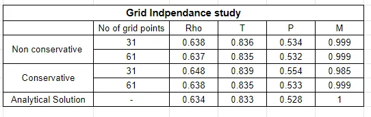
1.As the number of grid points have been increased the solution is moving closer to the analytical solution
2.Since there is no significant change in values of variables after increasing the number of grid points the solution may be said to grid-independent.
3.Both conservative as well as Non-conservative approaches have produced satisfactory results. However non-conservative approach seems to produce slighlty more accurate results.
5.RESULTS
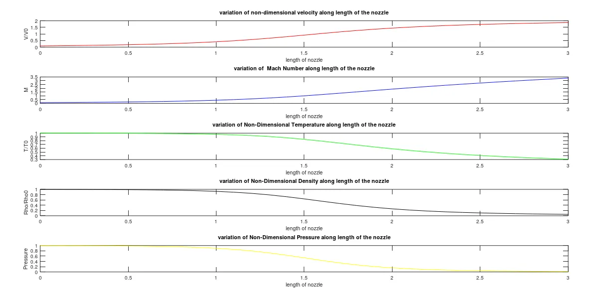
5.(a)Steady steady distribution of Primitive varaibles
Non-conservative
Conservative
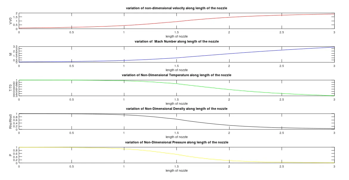
1.At the Entry of the nozzle Pressure,Density and Tempertaure are at Stagnation values i.e 1 while velocity and Mach number are nearly zero as velcocity is nearly zero.
This is consistent with the intial consitions given
2.Mach number at the throat of the nozzle(L=1.5) is 1.This is consistent with theory as mach number at throat is 1 in a supersonic nozzle
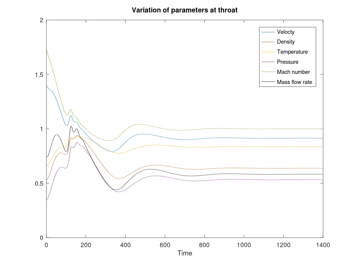
5.(b) Variation of primative variables at throat at different time steps
Non-Conservative
Conservative
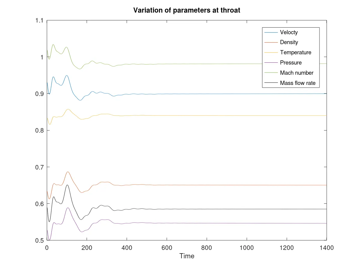
1.After 1000 Iterations the solution of both apporaches become stable
5.(c) Variation of mass flow rate at various time steps
Non Conservative
 Conservative
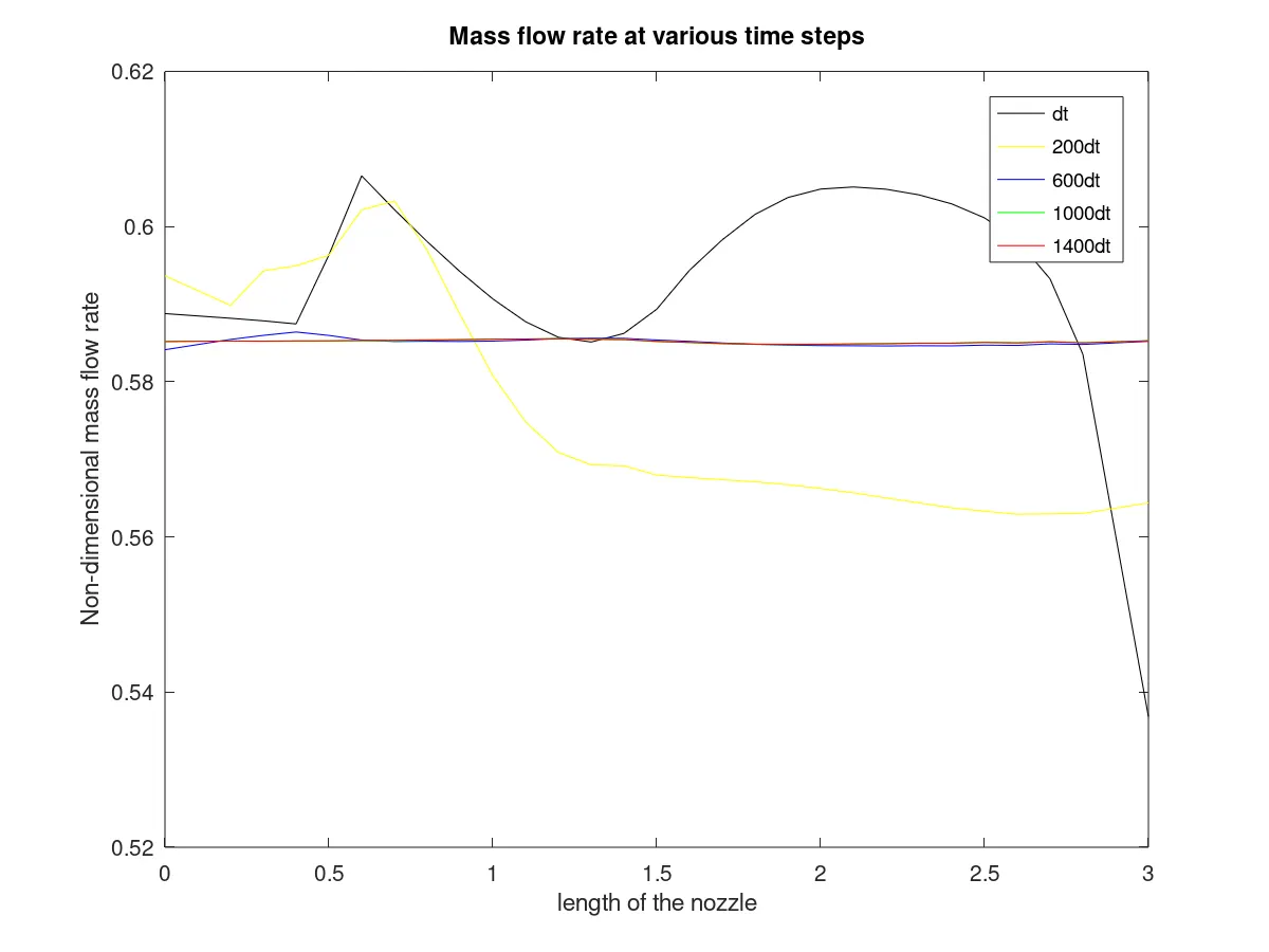
1.High variation in mass flow rate along the length of nozzle in initial time steps
2.Solution stabilizes at 600dt
3.High intial variation observed in non conservative approach. This is due to the fact that the conservative approach is better at conserving mass
5.(d) Comparison of normalized mass flow rate of both forms at steady state
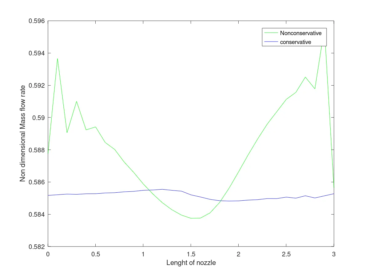
1.High variation of mass flow rate along the length of the nozzle observed in non-conservative form. In constrast there is minimal variation of mass flow rate in conservative form.
The conservative aprroach is better at conserving mass.
6.CONCLUSION
The simulation is completed with satisfactory results obtained for both approaches. The conservative approach was more tedious to solve and program. However it produces better results in terms of mass flow distribution. The non-conservative form on the other hand was easier to code and in general produced slightly more accurate results than the conservative form