Week 5 - Mid term project - Solving the steady and unsteady 2D heat conduction problem
1.PROBLEM
To Solve the 2D heat conduction equation by using the point iterative techniques. The Boundary conditions for the problem are as follows;
Top Boundary = 600 K
Bottom Boundary = 900 K
Left Boundary = 400 K
Right Boundary = 800 K
The following iterative methods will be used
1. Jacobi
2. Gauss-seidel
3. Successive over-relaxation
absolute error criteria - 1e-4
2.THEORY
Heat transfer is the phenomenon where transfer of energy occurs by virtue of Temperature difference.
Heat transfer occurs through 3 modes
a)Conduction-Heat transfer betwwen two bodies or two parts of a body where molecules are stationary
b)Covection- Heat transfer between a moving fluid and a solid body
c)Radiation-Heat transfer by measnof radiation
The problem given is that of condution with no internal heat generation
Steady State Analysis
Steady state is defined as the state where the change in parameters with respect to time are zero or negligible
Transient Analysis
Transient state is the state where where the change in parameters with respect to time are non-zero and not negligible
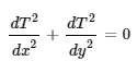
The Heat conduction equation for steady state analysis is
The Transient Heat conduction equation is
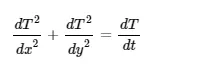
The above two equations must be solved for various cases to get the required tempertature distribution
3.PROGRAMS
3.(a) Program for steady state analysis
clc
clear all
%Inputs
nx=10;
ny=10;
T=ones(ny,nx);
x=linspace(0,1,nx);
y=linspace(0,1,ny);
dx=1/nx;
dy=1/ny;
k=2*((dx)^2+(dy)^2)/((dx)^2*(dy)^2);

%Index
m=3;
%Error
e=1e3;
%Initial Condtions
for i=1:nx
  for j=1:ny
    T(i,j)=300;
  endfor
endfor
%Boundry conditions
T(nx,:)=900 ;
T(:,nx)=800;
T(:,1)=400;
T(1,:)=600;
T(nx,1)=(900+400)/2;
T(nx,nx)=(800+900)/2;
T(1,nx)=(800+600)/2;
T(1,1)=(600+400)/2;
Told=T;
jacobiiter=0;
gs_iter=0;
SOR_iter=0;
%Jacobi Method
if m==1
  while e>1e-4
    for i=2:nx-1
      for j=2:ny-1
        T(i,j)=(1/k)*((Told(i+1,j)+Told(i-1,j))/(dy)^2)+(1/k)*((Told(i,j+1)+Told(i,j-1))/(dy)^2) ;
      endfor
    endfor
    e=max(max(abs(Told-T)));
    Told=T;
    jacobiiter=jacobiiter+1;
  endwhile
  k='Jacobi'
endif
%Gauss-Seidel Method
if m==2
  while e>1e-4
    for i=2:nx-1
      for j=2:ny-1
        T(i,j)=(1/k)*((T(i+1,j)+T(i-1,j))/(dy)^2)+(1/k)*((T(i,j+1)+T(i,j-1))/(dy)^2) ;
      endfor
    endfor
    e=max(max(abs(Told-T)));
    Told=T;
    gs_iter=gs_iter+1;
  endwhile
  k='Gauss'
endif
%SOR Method
%Relaxation factor
a=1.2
if m==3
  while e>1e-4
    for i=2:nx-1
      for j=2:ny-1
        T(i,j)=(1-a)*Told(i,j)+a*((1/k)*((T(i+1,j)+T(i-1,j))/(dy)^2)+(1/k)*((T(i,j+1)+T(i,j-1))/(dy)^2));
      endfor
    endfor
    e=max(max(abs(Told-T)));
    Told=T;
   SOR_iter=SOR_iter+1;
   iter=SOR_iter;
  endwhile
  k='SOR'
endif
%Plotting
[M,N]=contourf(x,y,T)
clabel(M,N)
colormap(jet)
colorbar
set(gca,'ydir','reverse')
title(k)
xlabel('x-axis')
ylabel('y-axis')
3.(b) Program for Transient Analysis -Explcit
clc
clear all
%Inputs
nx=10;
ny=10;
T=ones(ny,nx);
x=linspace(0,1,nx);
y=linspace(0,1,ny);
dx=1/nx;
dy=1/ny;
alpha=1.5;
dt=0.001
k1=(alpha*dt)/((dx)^2)
k2=(alpha*dt)/((dy)^2)
%Index
m=1;
%Initial Condtions
for i=1:nx
  for j=1:ny
    T(i,j)=300;
  endfor
endfor
%Boundry conditions
T(nx,:)=900 ;
T(:,nx)=800;
T(:,1)=400;
T(1,:)=600;
T(nx,1)=(900+400)/2;
T(nx,nx)=(800+900)/2;
T(1,nx)=(800+600)/2;
T(1,1)=(600+400)/2;
Told=T;
Explicit_iter=0
%Explicit Iterations
if m==1
  while e>1e-4
    for i=2:nx-1
      for j=2:ny-1
        T(i,j)=Told(i,j)+(k1)*(Told(i+1,j)-2*Told(i,j)+Told(i-1,j))+(k2)*(Told(i,j+1)-2*Told(i,j)+Told(i,j-1)) ;
      endfor
    endfor
    e=max(max(abs(Told-T)));
    Told=T;
    Explicit_iter=Explicit_iter+1;
  endwhile
endif
%Plotting
[M,N]=contourf(x,y,T)
clabel(M,N)
colormap(jet)
colorbar
set(gca,'ydir','reverse')
title('Transient analysis -Explicit')
xlabel('x-axis')
ylabel('y-axis')
3.(c) Transient Analysis -Implicit
clc
clear all
%Inputs
nx=10;
ny=10;
T=ones(ny,nx);
x=linspace(0,1,nx);
y=linspace(0,1,ny);
dx=1/nx;
dy=1/ny;
alpha=1.5;
dt=0.001;
k1=(alpha*dt)/((dx)^2);
k2=(alpha*dt)/((dy)^2);
nt=1400
%Index
m=3;
%Error
e=1e3;
%Initial Condtions
for i=1:nx
  for j=1:ny
    T(i,j)=300;
  endfor
endfor
%Boundry conditions
T(nx,:)=900 ;
T(:,nx)=800;
T(:,1)=400;
T(1,:)=600;
T(nx,1)=(900+400)/2;
T(nx,nx)=(800+900)/2;
T(1,nx)=(800+600)/2;
T(1,1)=(600+400)/2;
Told=T;
jacobiiter=0;
gs_iter=0;
SOR_iter=0;
Tprev=T
%Jacobi Method
if m==1
for t=1:nt
  e=1e3
 while e>1e-4
    for i=2:nx-1
      for j=2:ny-1
        term1=(1/(1+2*k1+2*k2));
        term2=k1*term1;
        term3=k2*term1;
         H=(Told(i-1,j)+Told(i+1,j));
         V=(Told(i,j-1)+Told(i,j+1));
         T(i,j)=term1*Tprev(i,j)+term2*H+term3*V;
      endfor
    endfor
    e=max(max(abs(Told-T)));
    Told=T;
    jacobiiter=jacobiiter+1;
  endwhile
 Tprev=T;
endfor
k='jacobi'
endif
%Gauss-Seidel Method
if m==2
  for t=1:nt
    e=1e3
  while e>1e-4
    for i=2:nx-1
      for j=2:ny-1
        term1=(1/(1+2*k1+2*k2));
        term2=k1*term1;
        term3=k2*term1;
         H=(T(i-1,j)+T(i+1,j));
         V=(T(i,j-1)+T(i,j+1));
         T(i,j)=term1*Tprev(i,j)+term2*H+term3*V;
      endfor
    endfor
    e=max(max(abs(Told-T)));
    Told=T;
    gs_iter=gs_iter+1;
  endwhile
  Tprev=T
endfor
k='Gauss-Seidel'
endif
%SOR Method
%Relaxation factor
a=1.2
if m==3
  for t=1:nt
    e=1e3
  while e>1e-4
    for i=2:nx-1
      for j=2:ny-1
        term1=(1/(1+2*k1+2*k2));
        term2=k1*term1;
        term3=k2*term1;
         H=(T(i-1,j)+T(i+1,j));
         V=(T(i,j-1)+T(i,j+1));
         T(i,j)=(1-a)*Told(i,j)+a*(term1*Tprev(i,j)+term2*H+term3*V);
      endfor
    endfor
    e=max(max(abs(Told-T)));
    Told=T;
   SOR_iter=SOR_iter+1;
  endwhile
  Tprev=T;
endfor
k='SOR'
endif
%Plotting
[M,N]=contourf(x,y,T)
clabel(M,N)
colormap(jet)
colorbar
set(gca,'ydir','reverse')
title(k)
xlabel('x-axis')
ylabel('y-axis')
4.RESULTS
4.(a)Steady state analysis
Jacobi Method
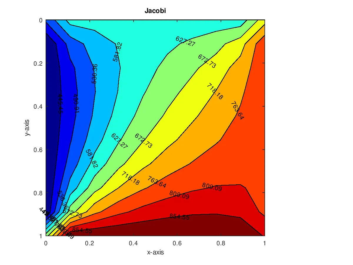
Number of iterations required =207
Gauss Seidel Method
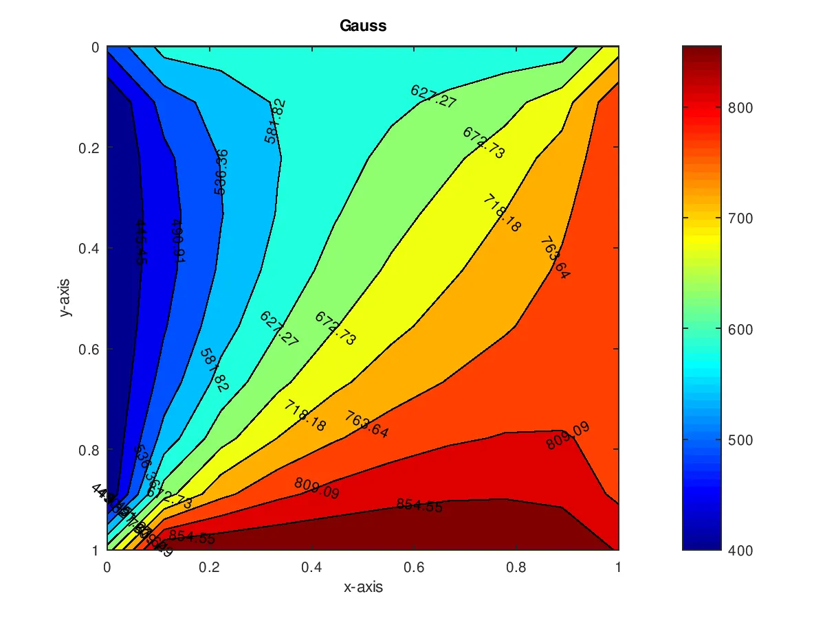
NNumberof iterations-111
3.SOR Method
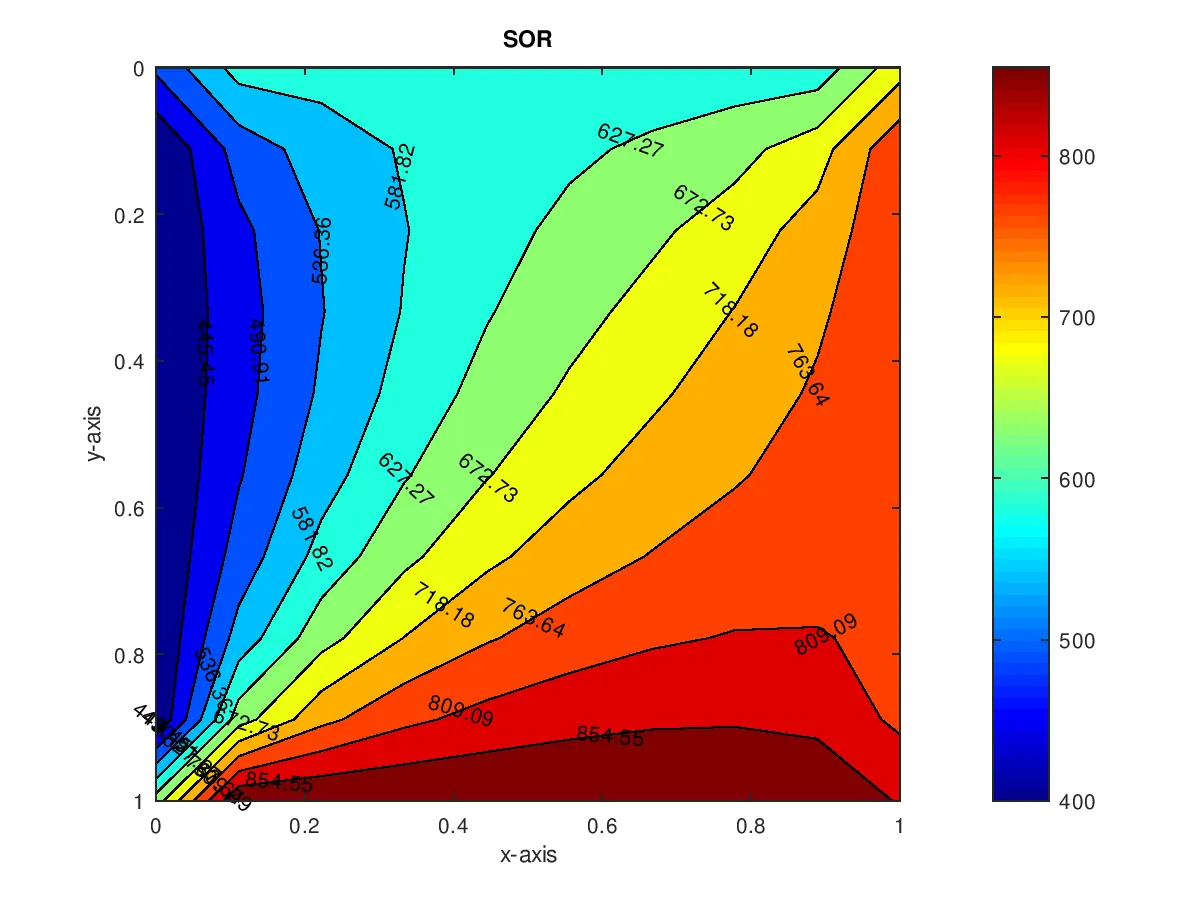
Number of iterations required-75
Transient-Explicit
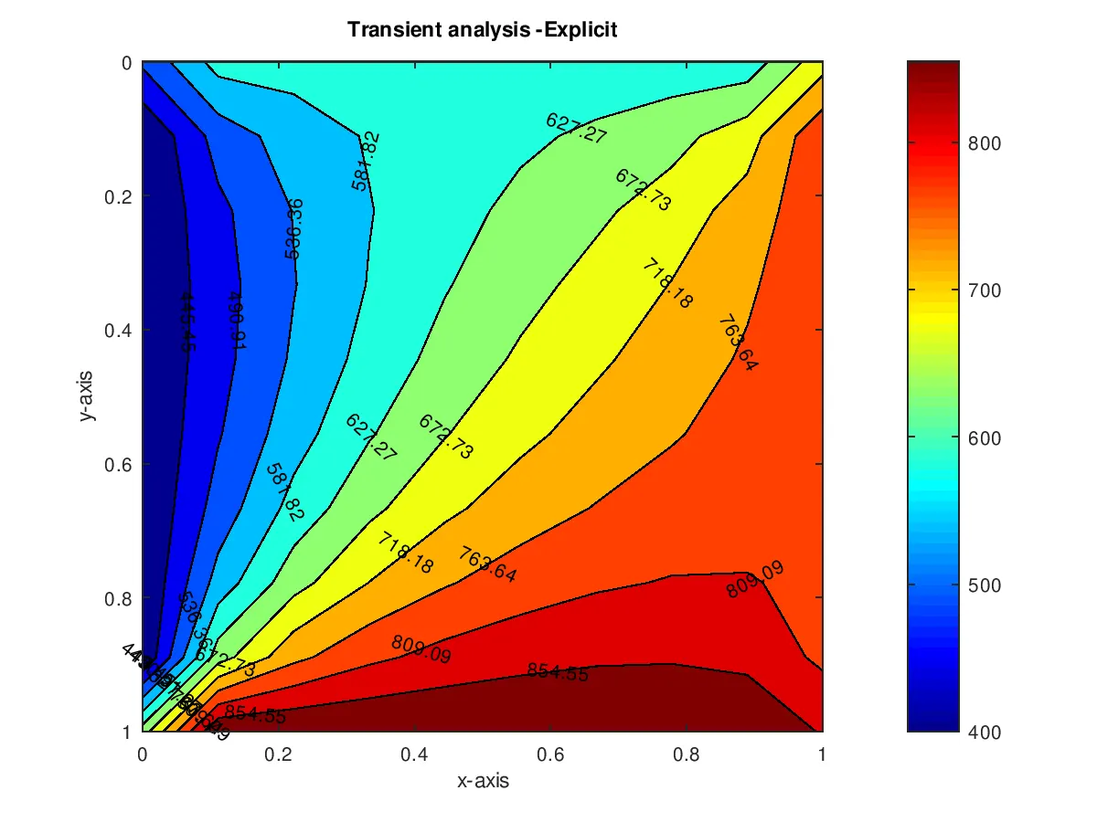
Number of iterations-334
4.(c) Transient Analysis -Implicit
Jacobi Method
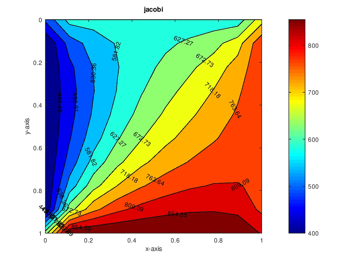
Number of iterations-3458
Gauss Seidel Method
Number of Iterations-2918
SOR Method
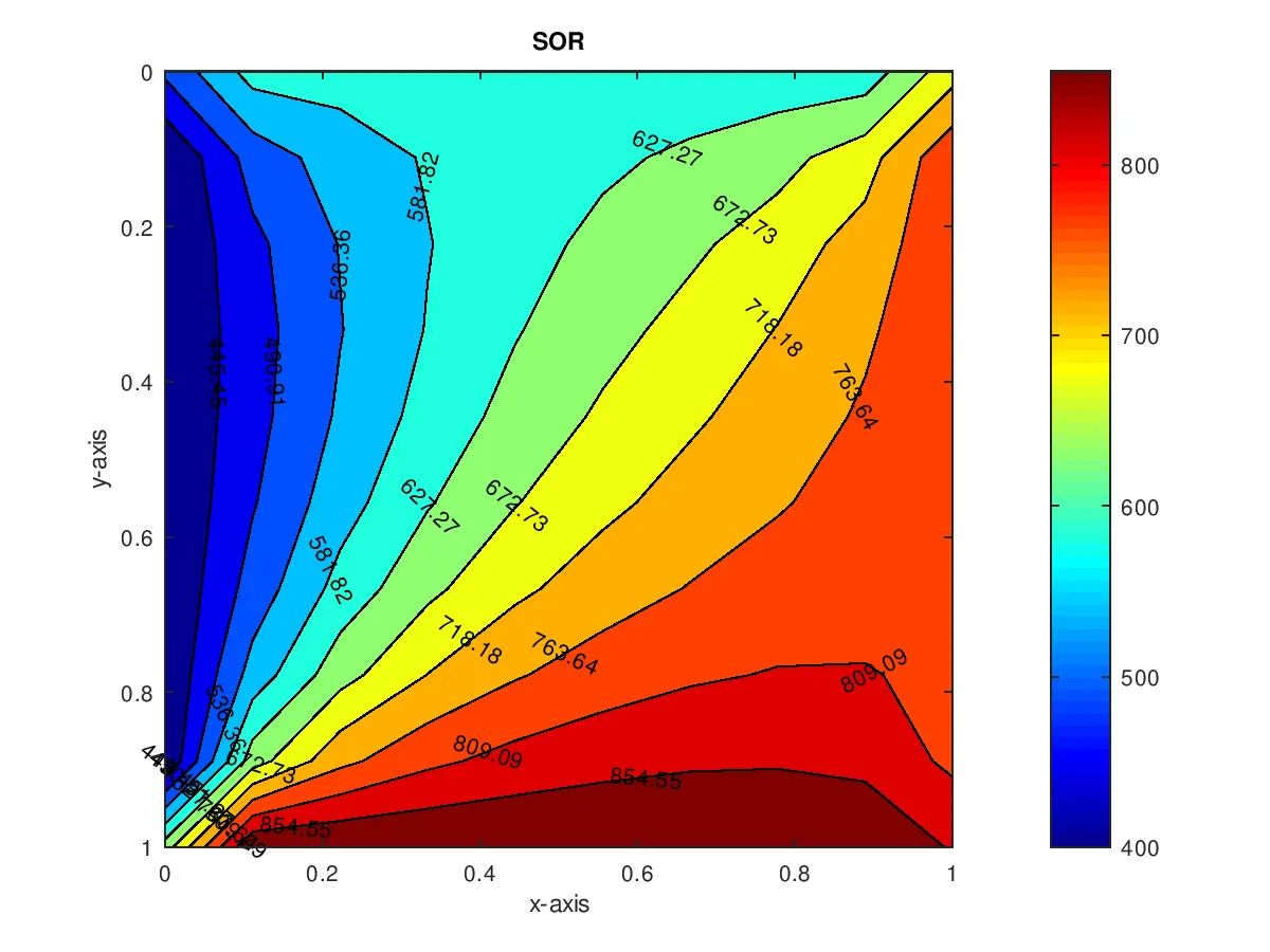
Number of iterations-2687
5.CONCLUSION
1.The following trend was observed with respect to number of iterations
Steady State simulation
Jacobi>Gauss Seidel>SOR
Transient Simulation
Jacobi>Gauss Seidel>SOR
Overall
Jacobi-Transient>Gauss Seidel-transient>SOR-Trasnient>Explicit-Trasnient>Jacobi-steady>Gauss Seidel-Steady>SOR-Steady
2.The SOR method proves to require the least amount of iterations in comparison with the Gauss-Seidel and Jacobi method