Week 9 - FVM Literature Review

AIM:- To Study the Finite Volume Method and Finite Difference Method and describe the need for interpolation schemes and flux limiters in FVM, Also Explain 1D linear heat conduction equation as an example.

INTRODUCTION:-

Basically Descritization Methods are divided in to Three types as Follows.

• Finite Diffrence Method:-

The finite difference method relies on discretizing a function on a grid. To use a finite difference method to approximate the solution to a problem, one must first discretize the problem's domain. This is usually done by dividing the domain into a uniform grid.

SOURCE:- en.wikipedia.org/wiki/Finite_difference_method

• Finite Volume Method:-

The finite volume method (FVM) is a method for representing and evaluating partial differential equations in the form of algebraic equations. In the finite volume method, volume integrals in a partial differential equation that contain a divergence term are converted to surface integrals, using the divergence theorem. These terms are then evaluated as fluxes at the surfaces of each finite volume. Because the flux entering a given volume is identical to that leaving the adjacent volume, these methods are conservative. Another advantage of the finite volume method is that it is easily formulated to allow for unstructured meshes. The method is used in many computational fluid dynamics packages. "Finite volume" refers to the small volume surrounding each node point on a mesh.

SOURCE:- https://en.wikipedia.org/wiki/Finite_volume_method

• Finite Element Method:-

The finite element method (FEM) is a popular method for numerically solving differential equations arising in engineering and mathematical modeling. Typical problem areas of interest include the traditional fields of structural analysis, heat transfer, fluid flow, mass transport, and electromagnetic potential.

The FEM is a general numerical method for solving partial differential equations in two or three space variables (i.e., some boundary value problems). To solve a problem, the FEM sub-divides a large system into smaller, simpler parts that are called finite elements.

SOURCE:- https://en.wikipedia.org/wiki/Finite_element_method

Drawbacks of Finite Difference Method:-

• In FDM we can not calculate Complex Geometry Problem Mesh, due to not aligned into X,Y and Z Direction.
• Due to mis-alignment we can not calculate Proper adjecent Node, due to which finding Mesh is Difficult, we can over-Come this by using Correction Factor,but its Time Consuming Process.
• For Complex Profiles This method is less Preffered.

• Finite Volume Method:-

The finite volume method (FVM) is a method for representing and evaluating partial differential equations in the form of algebraic equations. In the finite volume method, volume integrals in a partial differential equation that contain a divergence term are converted to surface integrals, using the divergence theorem. These terms are then evaluated as fluxes at the surfaces of each finite volume. Because the flux entering a given volume is identical to that leaving the adjacent volume, these methods are conservative. Another advantage of the finite volume method is that it is easily formulated to allow for unstructured meshes. The method is used in many computational fluid dynamics packages. "Finite volume" refers to the small volume surrounding each node point on a mesh.

In Finite Volume Method we can write equation on over full Domain instead of single point. so inside domain Flow is Conserved and we can calculate all properties with all perticular Volume. we uses Integral form for Solving Governing Equation.

STEPS for Solving FVM Problem:-

1. First Write down the 1D Liniear Heat Convection equation, then Integrate the Form of equation.

2. Apply Gauss Divergence Theorem.

3. we can get the Descritized form then we can calculate this.

Consider the Steady state Conduction Equation.

`del/(delx)(alpha*(delT)/(delx))+S=0`

Where,

`alpha=`Thermal Diffussivity Term.

`(delT)/(delx)`= Temperature Gradient along X Direction.

S= Source Term.

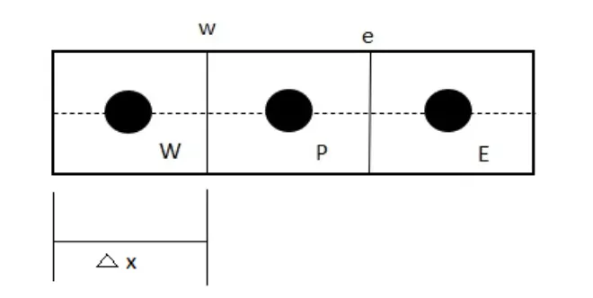
The Governing equation `del/(delx)(alpha*(delT)/(delx))+S=0` is vallid at every point in Domain means entire Volume.

we consider small Control volume and multyplied governing equation and integrate it for control volume thet should be equal to zero so integral form of equation.

we take the conservation equation is vallid at single point thus vallideted to entire volume, so prperties are conserved.

Multiplying the equation by dv and integrate,

`int(del/(delx)(alpha*(delT)/(delx))+S)dv=0`

`intdel/(delx)(alpha*(delT)/(delx))dv+intSdv=0`

since, `dv=A*dx`

`intdel/(delx)(alpha*(delT)/(delx))A*dx+intSdv=0`

`[alpha*A*(delT)/(delx)]_w^e +overlineSdv=0`

`overlineS=`avrage of Source term.

`alpha_e*A(delT)/(delx_e)- alpha_w*A(delT)/(delx_w) +overlineSdv=0`

if `alpha=`Constant.

`alpha*A[(T_e-T_p)/(Deltax)]-alpha*A[(T_p-T_w)/(Deltax)]+ overlineSdv=0`

The Source term which is added in cell, if this is function of it we have to linearize it, so `overlineStoS_u+S_pT_p`

{Heat Flux}out-{Heat Flux}in+Source Term=0

`alpha*A[(T_e-T_p)/(Deltax)]-alpha*A[(T_p-T_w)/(Deltax)]+ overlineSdv=0`

The ammount of heat is Removed is Conservred.

Different Schemes Used to solve Equation.

1. Gradient Schemes.

2. Interpolation Schemes.

1. Gradient Schemes:-

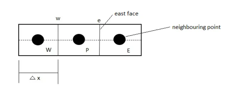
Calculating the Temperature at east face we used neighbouring Point, this presents Numeriacal gradient is called Gradient Schemes.

2. Interpolation Schemes:-

In this Scheme in Finite Volume Formation Integral required some unknown variables at control volume. this values are obtained by deploying some interpolation Schemes.

let us consider the case of stedy stete convection and Diffusion.

`d/(dx)(rhouphi)=(d)/(dx)(Gamma(dphi)/(dx))`

where `phi`is solution variable (scaler),

`rho` is Density

`u` is Velocity

`Gamma` is Diffusion Coeifficient.

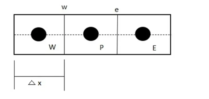
The above fig shows the three nighbouring points ( control volumes) which is then derrived for discritized.

Integrating the governing equation for control volume around Grid point 'P'

`(rhouphi)_e-(rhouphi)_w=(Gamma(dphi)/(dx))_e-(Gamma(dphi)/(dx))_w`

Evaluation of Left hand side require the value of `phi`over the faces e and w these values are employing the certain interpolation schemes.

Types of Interpolation Schemes:-

1. Upwind interpolation Schemes

2. Linear Interpolation Schemes

3. Quadreadic Upwind Interpolation Schemes

4. Hybrid Schemes

5.Total Dimenstioning Variation Schemes

1. Upwind interpolation Schemes:-

The upward interpolation having the direction of the fluid flow and based on it the value of the solution variables at the face its value at upstream Computational node.

If the fluid flow from west to east (as per fig) then,

`phi_eapproxphi_P`

and fluid moving from east to west

`phi_eapproxphi_E`

2. Linear Interpolation Schemes:-

In this Scheme approximate the values of the variable at control volume face interpolating values linearly at two nearly computational nodes.

The linear interpolation is almost same as central diffrence of first order derivative . it is second order accurate and produces ocillatory solution and equation as below,

`f_e=f_Elamda_e+f_P(1-lamda_e)`

FLUX LIMITER:-

1. Flux Limiter used where to avoid the high resolution Oscillation developed due to Shocks,Dis-Contuinity and Sharp edges at domain.

2. Flux Limter used for keep the Bounded values at cell faces.

3. Flux Limiter protect solution From Overshoot.

Consider the 1D Semi descrit Schemes,

`(du_i)/(dt)+(1)/(Deltax_i)[F(u_(i+1/2))-[F(u_(i-1/2))]=0`

`F(u_(i+1/2)) and F(u_(i-1/2))`represents the edge fluxes for the `i^(th`cell can represented by low and High Resolution then flux limiter switch between these Schemes close to perticular cell.

`F(u_(i+1/2))=f^(low)(i+1/2)-phi(ri)(f^(low(i+1/2))-f^(high(i+1/2)))`

`F(u_(i-1/2))=f^(low)(i-1/2)-phi(ri-1)(f^(low(i-1/2))-f^(high(i-1/2)))`

Where,

`f^(low)`= Low Resolution Flux

`f^(high)`=High Resolution Flux

`phi(r)=` Flux Limiter Function

r = Ratio of successive gradient on Solution Mesh= `ri=(u_i-u_(i-1))/(u_(i+1)-u_i)`

`phi(r)ge0` = limiter function case

if limiter function=0 then low Resolution and sharp gradient.

if limiter function `gt` then High resolution and High gradient.

References:-

1. en.wikipedia.org/wiki/Finite_difference_method

2. https://en.wikipedia.org/wiki/Finite_volume_method

3. https://en.wikipedia.org/wiki/Finite_element_method