Week 3 - Solving second order ODEs

Aim: To solve Second Order Ordinary Equation and To Describe the Transient behaviour of Simple Pendulum.

Objective: Write a program in Matlab to solve ODE and simulate the Simple pendulum motion.

Governing Equation:

`(d^2theta)/(dt^2)+(b/m)*(d*theta)/(dt)+g/l*sintheta=0`

Where,

b= Damping Coeficient;

m= mass in kg ;

g= Accleration due to gravity `m/s^2`

L= Length of Pendulum in m;

Theory:

Simple Pendulam

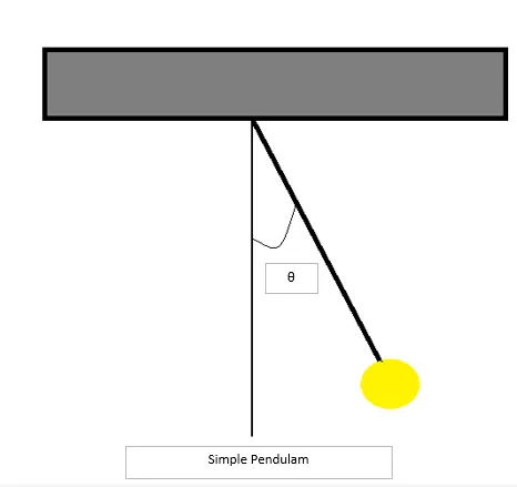
Fig. Simple Pendulam

Above Fig Shows that Simple pendulam having Below Parameters.

length of string (L) = 1 m;

ball mass (m)= 1 kg;

Angle = `theta`

Damping Coefficient= 0.05;

acceleration due to gravity 'g'=9.81 m/s^2

in fig We can see one end of pendulam is Fixed and another is Free, having one spherical ball having mass m, Length of the string (L) having damping Coefficient 0.05 and accelaration due to gravity 9.81 m/s^2.

For Pragramming in MATLAB we have to Convert the Governing Equation into Second order to 1st order.

`(d^2theta)/(dt^2)+(b/m)*(d*theta)/(dt)+g/l*sintheta=0`

Assume,

`theta=theta1`

`(d.theta)/dt=(d.theta1)/dt=theta2`.........................................................................1

`(d^2theta)/(dt^2)=(d^2theta1)/(dt^2)=d/dt((d.theta1)/(dt))=d/dt(theta2)`....................2

`(d^2theta)/dt^2+b/m*(d.theta)/dt+g/lsintheta=0`

`(d^2theta1)/(dt^2)+b/m*(d.theta1)/(dt)+g/l.sintheta1=0`

`(d^2theta2)/(dt)+b/m*theta2+g/l.sintheta1=0`

`(d theta1)/dt=theta2`

`(d theta2)/dt =-(b/m).theta2-g/l.sintheta`

we can utilize this equation to Write Program.

Main Code:

% simple_pendulam_Simulation

clear all
close all
clc

% inputs

l=1;
m=1;
b=0.05;
g=9.81;

ctr=1;

% initial condition
theta_0=[0,3];

% Time

t_span=linspace(0,20,500);

% plotting angular displacement and angular velocity

% solving ODE
figure(1)
[t,results]=ode45(@(t,theta) odefun(t,theta,l,b,g,m),t_span,theta_0);
plot(t,results(:,1))
hold on 
plot(t,results(:,2))
xlabel('time')
ylabel('plot')
axis([0,20,-4,4])
legend('angular displacement','angular velocity');
hold off

% pendulam motion Animation

theta_p=results(:,1);

for i=1:length(theta_p)
    theta_p1=theta_p(i);

    x0=0;
    y0=1;

    x1= x0+1*sin(theta_p1);
    y1= y0-1*cos(theta_p1);

    % plot the pendulum
    figure(2)
    plot([-1 1],[1 1],'color','r','LineWidth',5);                                  % For fixed Support
    hold on
    plot([x0 x1],[y0 y1],'Color','k','linewidth',3);                               % For String
    plot(x1,y1,'o','markers',30,'MarkerFaceColor',[1 1 0],'MarkeredgeColor','b')   % markers used for Making Sphere Ball
    plot([0 0],[-0.3 1],'--','Color','k');                                         
    hold off

    axis([-1.5 1.5 -0.5 1.5])
    title('simple pendulam simulation')
    pause(0.0000020)

    M(ctr)=getframe(gcf);
    ctr=ctr+1;
end

%creating simulation by video file 

movie(M)
videofile=VideoWriter('simple pendulam.avi','Uncompressed AVI');
open(videofile)
writeVideo(videofile,M)
close(videofile)

Function Code:

function [dtheta_dt]=odefun(t,theta,l,b,g,m)
theta1=theta(1);
theta2=theta(2);
dtheta1_dt= theta2;
dtheta2_dt=-(b/m)*theta2-(g/l)*sin(theta1);
dtheta_dt=[dtheta1_dt; dtheta2_dt];
end

Program Code Explaination:

Step 1: First by function code we have to find Governing equation by using odefunc Command.

Step 2: 1. after that we can start new main code for Simple pendulam Simulation.

2. start from Clear all, close all and clc

3. then we have to write input parameters like,damping coefficient(b), mass(m),accleration due to gravity (g) and length l in (m);

4. Then we have to write initial conditions like angle Theta and Time span by using linspace command.

Step 3 : Then we have to solve ODE by using ode45 annoynomus Function and plot graph of angular displacement vs angular velocity.

Step 4: Then we have to write program about Pendulam motion animation by using for loop,

we have to find x0,y0,x1,y1 values,and then plot the figure(2), by using plot command we can draw Fixed support, then by using plot command plot the string ,and then finally by using markers command we plotted Ball. then we can fix axis by using axis command. by using (gcf) we can get correct frames.

Step 5: we have to Create Animation by using Movie Command.

Results:

Angular Displacement and Angular Velocity Plots:

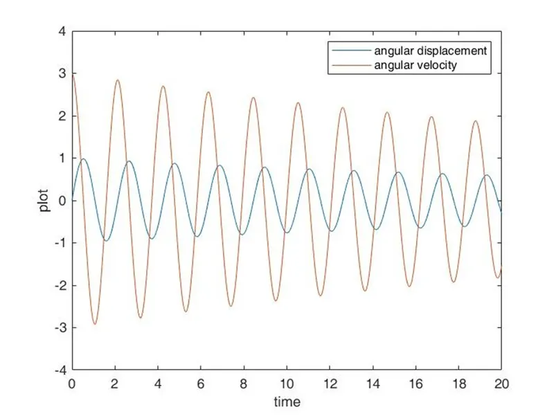
Fig. Angular Displacement and Angular Velocity Plots

Here in above Fig we can see how The behaviour of angular displacement and velocity changed with respect to time (20 sec). when pendulam start to displace (swing) the amplitude will be more but at the end point of the Time we can see Less Amplitude. like that we can see transient behaviour of Simple pendulam by using solving Second order ODE.

Errors While Running Programing:

Unrecognized function or variable 'theta_p1'.

Error in simple_pendulam (line 43)

x1=x0+1*sin(theta_p1);

After Correcting Variable thetap_1 to theta_p1 Error Removed and Program Run Successfully.

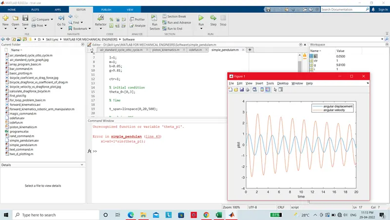
Fig. Errors While Running Programing

Conclusion:

1) From Angular Displacement and Angular Velocity Graph we concluded that as Damping is happened in Simple Pendulam we can see the transient behaviour in Angular Displacement and Angular Velocity.

2) We concluded that By Solving Second order ODE, we can Run program Successfully and made Animation of Simple Pendulam and we can see behaviour of Angular Displacement and Angular Velocity.

3) Video Link is attached Below to Show Video.

Follow the link to Show Video:https://youtu.be/PuhKuiDPHQ4