Week 9 - FVM Literature Review

Finite Volume Method:

 Finite Volume Method is a numerical method used for solving Partial Differential Equations, particularly for fluid flows, numerically. It involves 3 crutial steps with following order:

1. Grid Generation
2. Integration
3. Interpolation functions: Making a profile assumption for dependent variable for evaluating integrals obtained in the above step and obtaining results in form of algebric equations.

Grid Generation:

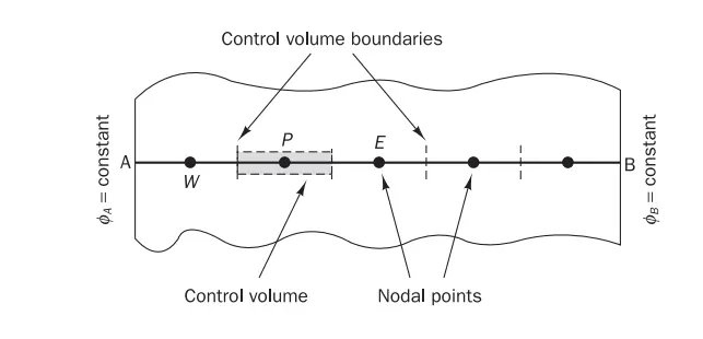
The domain is divided into finite-sized sub-domains. With each sub-domain represented by finite number of grid points. While any point in the sub-domain or 'control volume' can be considered as the representative point, choosing 'geometric centers' as the the representative point is a convention people follow. It is  common practice to set up control volumes near the edge of the domain in such a way that the physical boundaries coincide with the control volume boundaries. An illustration is shown below:

Integration:

Integrating the governing differential equation over each sub-domain. Since differential equation in differential form is valid over a point, when integrated over the sub-domain we are implying that the conservation principle is expanded to the entire sub-domain in an integral sense. This is why FVM is accepted by entire fluid and heat transfer community because of its own implimentation of conservativeness.

Interpolation Function:

To convert the derivative terms into algebric terms we assume profile function for dependent variable i.e: we choose a function of how the dependent variable will vary from one control volume to the adjacent control volume. This chosen or assumed profile function is called Interpolation Function. Choosing a higher degree polynomial as Interpolation function may or may not give more accurate results. It all boils down to how well the function behaves numerically i.e: if it accomodates all the basic physical requirements like continuity of fluxes at the surfaces.

Types of Interpolation functions:

1. Linear Interpolation
2. Upwind Interpolation
3. Quadratic Upwind Interpolation
4. Hybrid, TVD and ENO Interpolation

Considering 1D Steady State Heat Conduction with constant Source term in a uniform sized horizontal rod, the governing differential equation is given by:

`del/(delx) [k(delT)/(delx)] +S=0` with k and S as constants.

1.  Dividing the domain in multiple sub-domains,

The length of each control volume is `delx`with nodes at the geometric center of each element. The boundary temperatures being `T_A and T_B`. 

2. Integrating the governing Differential equation over each control volume,

`intdel/(delx) [k(delT)/(delx)]dV +intS.dV=0`

Using divergence theorem and evaluating the integral,

`[kA(delT)/(delx)]_e- [kA(delT)/(delx)]_w +SDeltaV=0` where subscripts 'e' and 'w' refers to the node of control volumes to the immediate right and left of the node for which we are writing the equation respectively.

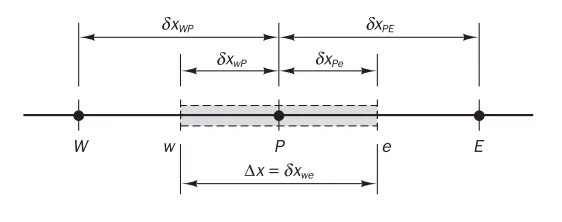
3. Assuming 'T' to vary in a piecewise linear manner from grid point to grid point for e.g.: `(delT)/(delx)=(T_P-T_W)/(deltax)` this assumed 'T' is a type of Interpolation Function. A linear profile assumption is called a linear interpolation function.

`Since, values for T is known for neighbouring nodes i.e: node 2 to node 4, `[k_e/(deltax_(PE))A_e+k_w/(deltax_(WP))A_w]T_P=[k_w/(deltax_(WP))A_w]T_W+[k_e/(deltax_(PE))A_e]T_E +SADeltax` is discretized equation for nodes from node 2 to node 4.`

Flux limiter -WikipediaAs `A_e=A_w=A and k_e=k_w=k` .Writing the above equation as  `a_PT_P=a_ET_E+a_WT_W+b` where,

`a_P`	`a_E`	`a_W`	b
`a_W+a_E`	`k/(deltax)A`	`k/(deltax)A`	`SADeltax`

For boundary node 1:
`kA[(T_E-T_P)/(deltax)]+kA[(T_P-T_A)/((deltax)/2)]+=0`. Similar expression is obtained for boundary node 5.

The equations obtained are solved explicitly or implicitly to obtain values for the flow field.

Flux Limiter:

Also referred to as slope limiter as they have the effect of limiting solution gradient near shocks and discontinuities. They are used to avoid spurious oscillations that otherwise occur with high order spatial discretization schemes due to shocks, discontinuities and sudden chaange in solution domain.

It is represented by `phi(r)` and is constrained to be `>=0`where 'r' represents the ratio of successive gradients in solution.
`r_i=(T_i-T_(i-1))/(T_(i+1)-T_i)`  here  T represents the dependent variable.
If `phi(r)=0` it represents sharp gradients, opposite slopes or zero gradient. The flux is represented by low resoluion scheme.
If `phi(r)=1` it represents high resolution scheme.
'resolution' term is used in the meaning of accuracy of the solution.

Some commonly used Flux Limiter functions are:

1. CHARM
2. SUCS
3. HQUICK
4. UMIST etc.

Difference between FVM, FEM and FDD:

Just like Finite Difference Method (FDM),  Finite Element Method (FEM) and Finite Volume Method (FVM) are numerical methods for solving Partial Differential Equations numerically.

In FDM, the domain is divided into number of sub-domains in the meaning of discrete grid points. Whereas in FEM the domain is divided into number of sub-domains in the meaning of elements i.e.: in FEM an algebric equation is formed from PDE for each element and not the entire domain primarily.

In FVM, similar to FEM, the domain is divided into number of sub-domains with each sub-domain represented by finite number of grid points.

Why use FVM over FEM and FDM in CFD?

The answer is, though FEM is mathematically rigourous and can handle complex geometry with ease, it doesn't carry the property of 'conservativness' explicitly through its interpretation of fluid flow and 'heat and mass' transfer. FDM too doesn't guarantee conservativeness of physical quantities over the entire domain. Also FDM is not convinient to use while dealing with complex geometries. 

Refernces:

1. Interploation_scheme_NPTEL
2. Flux_limiter_wikipedia