Week 4.1 - Genetic Algorithm
Stalagmite Function:
Stalagmite refers to an upward-growing natural structures formed due to mineral deposits that precipitates from the water dripping onto the floor of the cave.
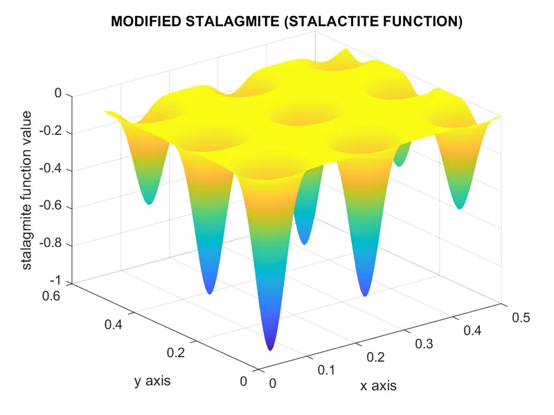
The stalagmite function when plotted on a 3d graph have the similar appearance and hence the name.
The problem statement asks for optimization of this function using genetic algorithm.But genetic algorithm in MATLAB inherently minimizes a function. Hence if optimization is carried out on stalagmite function as it is, it will always return zero as the solution and not the values at the peaks. As peaks in stalagmite function represents the maxima and not the minima.
So, in order to use genetic algorithm on stalagmite function we need to modify the stalagmite function so the peaks that represents maxima should represent minima instead.
This can be done by inverting the sign of stalagmite function i.e. instead of actual output of the function we will consider the negative value of the output instead. We might instead call it as 'stalactite function' as it will represent an inverted structure of stlagmite which is called 'Stalactite'.
1) The below program generates only a single iteration of GA for the modified stalagmite function:
close all
clear all
clc

%Genetic algorithm for maximizing stalagmite function (single iteration):

%%
x=linspace(0,0.5,150);                                 %workspace (x and y coordinates) for stalagmite function.
y=linspace(0,0.5,150);
[xx,yy]=meshgrid(x,y);                                 %generating meshgrid from above workspace.
for i=1:length(xx)                                     %calculating stalagmite function value for above workspace.
    for j=1:length(yy)
        inputs(1)=xx(i,j);
        inputs(2)=yy(i,j);
        f(i,j)=stalagmite_function(inputs);
    end
end

figure('Name','Stalagmite Plot')                        %plotting stalagmite and ga results.
surf(xx,yy,f)                                           %stalagmite surface plot as contour plot.
xlabel('x axis')
ylabel('y axis')
zlabel('stalagmite function value')
title('MODIFIED STALAGMITE (STALACTITE FUNCTION)')

shading interp
[input_opt, fval]=ga(@stalagmite_function,2)
1a)Below program is for Stalagmite function:
%Modified Stalagmite Function.
function [f] = stalagmite_function(inputs)
f1=(sin(5.1*pi*inputs(1)+0.5)).^6;
f2=(sin(5.1*pi*inputs(2)+0.5)).^6;
f3=exp((-4*log(2)*(inputs(1)-0.0667)^2)/0.64);
f4=exp((-4*log(2)*(inputs(2)-0.0667)^2)/0.64);
f=-f1*f2*f3*f4; %modifying stlagamite output by multiplying by -1 for ga to give maxima. 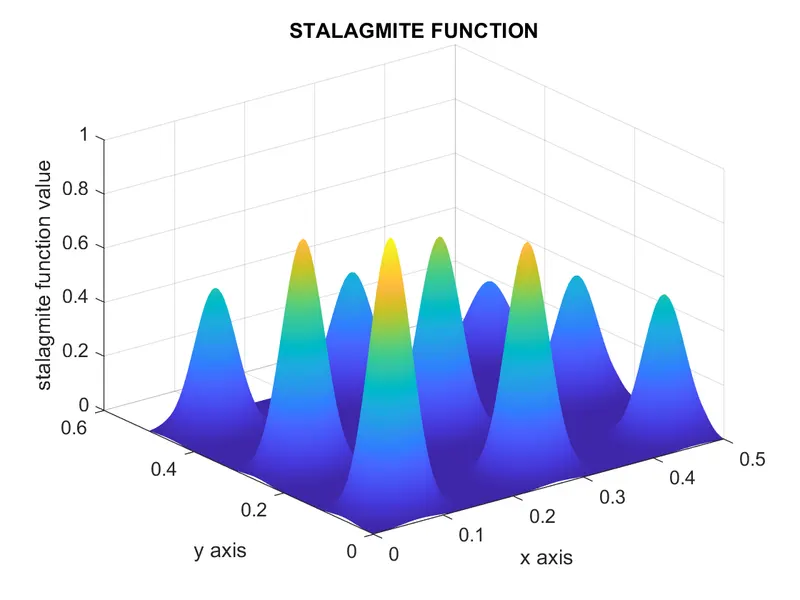
Genetic Algorithm:
It is a search-based optimization technique based on the theory of Genetics and Natural Selection.
It is frequently used to find optimal or near optimal solution of problems which are otherwise take a lifetime to solve using brute force or traditional methods. It is rigourously used in the fields of research and machine learing.
Optimization refers to finding the 'best solution' or 'set of best solutions' among all the possible solutions.
The definition of 'best' may vary from problem to problem. In mathematical terms it refers to maximization and minimization of one or more objective functions, which in our case is "Inverted Stalgamite or Stalactite Function".
The Genetic Algortihm is divided into 5 parts :
1) Population Initialization
2)Fitness function.
3)Crossover.
4)Mutation.
5)Survivor selection.
6)Return Best solution.
Population Initialization :
Population here is a subset of solutions in current generation. It can be selected randomly or based on some heuristics.While selection of population certain things have to be kept in mind -
a)The diversity of the population should be maintained to avoid premature convergence.
b)The population size should not be large enough as it can cause the GA to slow down but it should not be very samll either to avoid "not good enough" solutions.
Fitness Function :
A fitness function is defined as a function which takes a candidate solution to the problem as input and give output as how good the solution is with respect to the probelm in consideration.
In most cases of minimization and maximization problem the fitness function and objective function are the same.
Crossover :
More than one solution is selected and a new better solution is generated from it. The crossover is carried out with high probabiltiy.
Mutation :
Mutation refers to the random tweaks in the solution of following crossover. It is found that mutation is much more essential than crossover for the convergence of the solution. Higher the probability of the mutation more random will be the GA search for the best solution.
Survivor selection :
The new sets of solutions now form the parent solution and now are used for generating new and even better solutions.
The whole processes continues iteratively until we have our best solution or set of best solutions.
The syntax for GA in Matlab is :
x = ga(fun,nvars,A,b,Aeq,beq,lb,ub,nonlcon,intcon,options) where,
fun : represent the function to be optimized, which in our case, is stalagmite function.
nvars : represents the number of variables in the optimization function
A,b : represents the coefficients in the linear inequalities of the form Ax<=b
Aeq,beq : represents the coefficients in the linear equalities of the form Ax=b
lb,ub : represents the upper and lower bounds of the workspace for the GA
nonlcon : non linear constraints are provided.
intcon : constraints are given in integer form.
options : values in options replaces the default optimization parameters.
Advantages of GA over traditional gradient based methods:
1)faster than traditional methods in reaching in optimal solutions
2)provides a set of good solutions instead of one
3)doesn't require derivative information
4)useful when workspace and number of parameters are large
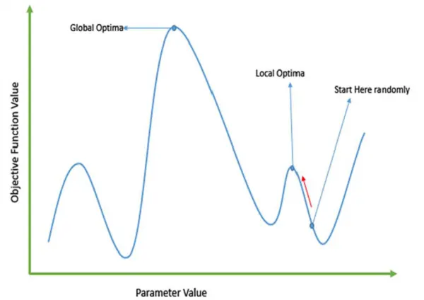
5)Traditional methods suffer from an inherent tendency of getting stuck at the local optima as shown in the following figure.
Limitations of GA:
1)Not suitable for simpler problems and for which derivative information is available as traditional methods will give more accurate and faster results.
2)Due to stochastic in nature there is no guarantee of optimality or quality of the solution.
3)If not implemented properly, the solution might not even converge.
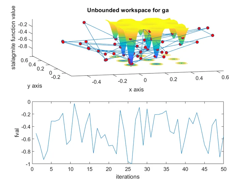
2)For unconditioned and conditioned ga with iterations:
close all
clear all
clc

%Genetic algorithm for maximizing stalagmite function for:
%1)unbounded workspace for ga and iterating it 50 times.
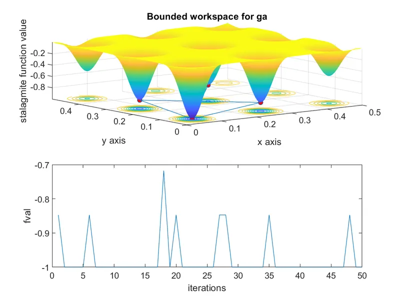
%2)bounded workspace for ga and iterating it 50 times.
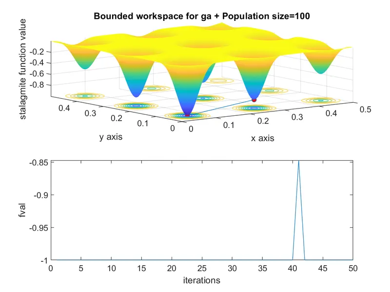
%3)bounded workspace for ga, population size of 100 and iterating it 50 times.

%%
%iterating genetic algorithm in unbounded work space.
x=linspace(0,0.5,150);                                 %workspace (x and y coordinates) for stalagmite function.
y=linspace(0,0.5,150);
[xx,yy]=meshgrid(x,y);                                 %generating meshgrid from above workspace.
for i=1:length(xx)                                     %calculating stalagmite function value for above workspace.
    for j=1:length(yy)
        inputs(1)=xx(i,j);
        inputs(2)=yy(i,j);
        f(i,j)=stalagmite_function(inputs);
    end
end

tic
figure(1)                                              %plotting stalagmite and ga results for unbounder workspace.
subplot(2,1,1)
hold on
surfc(xx,yy,f)                                         %stalagmite surface plot as contour plot.
shading interp
xlabel('x axis')
ylabel('y axis')
zlabel('stalagmite function value')
title('Unbounded workspace for ga')

numcases=50;
for i=1:numcases                                       %iterating ga 50 times
    [input_opt, fval]=ga(@stalagmite_function,2)
    x_iter2(i)=input_opt(1);
    y_iter2(i)=input_opt(2);
    fval_iter(i)=fval;
end
plot3(x_iter2,y_iter2,fval_iter,'-o','MarkerSize',5,'MarkerFaceColor','r') %plotting results for ga for 50 iterations.

subplot(2,1,2)                                                             %plotting output of ga vs iteration number.
plot(fval_iter)
xlabel('iterations')
ylabel('fval')
study1_time=toc

%%
%iterating genetic algorithm in bounded work space.
tic
figure(2)                                                                  %plotting stalagmite and ga results for unbounder workspace.
subplot(2,1,1)
surfc(xx,yy,f)
shading interp
xlabel('x axis')
ylabel('y axis')
zlabel('stalagmite function value')
title('Bounded workspace for ga')

hold on

numcase2=50;
for i=1:numcase2
    [input_opt2, fval2]=ga(@stalagmite_function,2,[],[],[],[],[0 0],[0.5 0.5]) %similar iteration of ga as case above with a slight difference i.e. bounding workspace.
    x_iter2(i)=input_opt2(1);
    y_iter2(i)=input_opt2(2);
    fval_iter2(i)=fval2;
end
plot3(x_iter2,y_iter2,fval_iter2,'-o','MarkerSize',5,'MarkerFaceColor','r')

subplot(2,1,2)
plot(fval_iter2)
xlabel('iterations')
ylabel('fval')
study2_time=toc

%%
%iterating genetic algorithm in bounded work space.
tic
figure(3)
subplot(2,1,1)
surfc(xx,yy,f)
shading interp
xlabel('x axis')
ylabel('y axis')
zlabel('stalagmite function value')
title('Bounded workspace for ga + Population size=100')

hold on
options=optimoptions('ga');                         %modifying ga conditions even further by changing default population size of 50 to 100.
options=optimoptions(options,'PopulationSize',100);

numcase3=50;
for i=1:numcase3
    [input_opt3, fval3]=ga(@stalagmite_function,2,[],[],[],[],[0 0],[0.5 0.5],[],[],options)
    x_iter3(i)=input_opt3(1);
    y_iter3(i)=input_opt3(2);
    fval_iter3(i)=fval3;
end
plot3(x_iter3,y_iter3,fval_iter3,'-o','MarkerSize',5,'MarkerFaceColor','r')

subplot(2,1,2)
plot(fval_iter3)
xlabel('iterations')
ylabel('fval')
study3_time=toc

%%
%Conclusion:
%Unbounded workspace results failed to converge & solution space is a mess.
%Bounded workspace give better result than unbounded case but still far from omptimized.
%Conditioning ga even further like increasing pouplation size provides near optimum results.
%But making these changes comes at a higher computational cost.
%So for reaching optimal solution one must first optimize their approach or procedure
%A compromise is to be made between optimization degree desired vs computational cost.