Week 3.5 - Deriving 4th order approximation of a 2nd order derivative using Taylor Table method

Taylor Table for Forward Difference Scheme:

F.D.S	f(i)	`Deltax`f'(i)	`Deltax^2f''(i)`	`Deltax^3f'''(x)`	`Deltax^4f''''(x)`	`Deltax^5f'''''(x)`	`Deltax^6f''''''(x)`
a`f_i`	a	0	0	0	0	0	0
b`f_(i+1)`	b	`b`	`frac{b}{2}`	`frac{b}{6}`	`frac{b}{24}`	`frac{b}{120}`	`frac{b}{720}`
c`f_(i+2)`	c	`2c`	`frac{4c}{2}`	`frac{8c}{6}`	`frac{16c}{24}`	`frac{32c}{120}`	`frac{64c}{720}`
d`f_(i+3)`	d	`3d`	`frac{9d}{2}`	`frac{27d}{6}`	`frac{81d}{24}`	`frac{243d}{120}`	`frac{729d}{720}`
e`f_(i+4)`	e	`4e`	`frac{16e}{2}`	`frac{64e}{6}`	`frac{256d}{24}`	`frac{1024e}{120}`	`frac{4096e}{720}`
g`f_(i+5)`	g	`5g`	`frac{25g}{2}`	`frac{125e}{6}`	`frac{625g}{24}`	`frac{3125g}{120}`	`frac{15625g}{720}`

Let `f_i''`=`af_i+bf_(i+1)+cf_(i+2)+df_(i+3)+ef_(i+4)+gf_(i+5)`

also from taylor table above:

`af_i=af_i`

`bf_(i+1)=bf_i+bDeltaxf_i'+b(Deltax^2)/2f_i''+b(Deltax^3)/6f_i'''+b(Deltax^4)/24f_i''''+b(Deltax^5)/120f_i'''''+O(Deltax^6)`

`cf_(i+2)=cf_i+c2Deltaxf_i'+c(4Deltax^2)/2f_i''+c(8Deltax^3)/6f_i'''+c(16Deltax^4)/24f_i''''+c(32Deltax^5)/120f_i'''''+O(Deltax^6)`

`df_(i+3)=df_i+d3Deltaxf_i'+d(9Deltax^2)/2f_i''+d(27Deltax^3)/6f_i'''+d(81Deltax^4)/24f_i''''+d(243Deltax^5)/120f_i'''''+O(Deltax^6)`

`ef_(i+4)=ef_i+e4Deltaxf_i'+e(16Deltax^2)/2f_i''+e(64Deltax^3)/6f_i'''+e(256Deltax^4)/24f_i''''+e(1024Deltax^5)/120f_i'''''+O(Deltax^6)`

`gf_(i-4)=gf_i+g5Deltaxf_i'+g(25Deltax^2)/2f_i''+g(125Deltax^3)/6f_i'''+g(625Deltax^4)/24f_i''''+g(3125Deltax^5)/120f_i'''''+O(Deltax^6`

since LHS only has `f''` term so equating sum of `f''` terms on LHS to RHS and equating sum of rest of similar terms equal to zero.

`sumcoeff.(f_i) =0`

`a+b+c+d+e+g=0` -[1]

`sumcoeff.(Deltaxf_i') =0`

`b+2c+3d+4e+5g=0` -[2]

`sumcoeff.(Deltax^2/2f_i'') =1`

`b+4c+9d+16e+25g=1` -[3]

`sumcoeff.(Deltax^3/6f_i''') =0`

`b+8c+27d+64e+125g=0` -[4]

`sumcoeff.(Deltax^4/24f_i'''') =0`

`b+16c+81d+256e+625g=0` -[5]

`sumcoeff.(Deltax^5/120f_i''''') =0`

`b+32c+243d+1024e+3125g=0` -[6]

Taylor Table for Central Difference Scheme:

C.D.S	f(i)	`Deltax`f'(i)	`Deltax^2f''(i)`	`Deltax^3f'''(x)`	`Deltax^4f''''(x)`	`Deltax^5f'''''(x)`	`Deltax^6f''''''(x)`
a`f_(i-2)`	a	-2a	`(4a)/2`	`(-8a)/6`	`(16a)/24`	`(-32a)/120`	`(64a)/720`
b`f_(i-1)`	b	`-b`	`frac{b}{2}`	`-frac{b}{6}`	`frac{b}{24}`	`-frac{b}{120}`	`frac{b}{720}`
c`f_(i)`	c	0	0	0	0	0	0
d`f_(i+1)`	d	`d`	`frac{d}{2}`	`frac{d}{6}`	`frac{d}{24}`	`frac{d}{120}`	`frac{d}{720}`
e`f_(i+2)`	e	`2e`	`frac{4e}{2}`	`frac{8e}{6}`	`frac{16d}{24}`	`frac{32e}{120}`	`frac{64e}{720}`

Let `f_i''=af_(i-2)+bf_(i-1)+cf_i+df_(i+1)+ef_(i+2)`

also from Taylor table above:

`af_(i-2)=af_i-a2Deltaxf_i'+a(4Deltax^2)/2f_i''-a(8Deltax^3)/6f_i'''+a(16Deltax^4)/24f_i''''-a(32Deltax^5)/120f_i'''''+O(Deltax^6)`

`bf_(i-1)=bf_i-bDeltaxf_i'+b(Deltax^2)/2f_i''-b(Deltax^3)/6f_i'''+b(Deltax^4)/24f_i''''-b(Deltax^5)/120f_i'''''+O(Deltax^6)`

`cf_i=cf_i`

`df_(i+1)=df_i+dDeltaxf_i'+d(Deltax^2)/2f_i''+d(Deltax^3)/6f_i'''+d(Deltax^4)/24f_i''''+d(Deltax^5)/120f_i'''''+O(Deltax^6)`

`ef_(i+2)=ef_i+e2Deltaxf_i'+e(4Deltax^2)/2f_i''+e(8Deltax^3)/6f_i'''+e(16Deltax^4)/24f_i''''+e(32Deltax^5)/120f_i'''''+O(Deltax^6)`

since LHS only has `f''` term so equating sum of `f''` terms on LHS to RHS and equating sum of rest of similar terms equal to zero.

`sumcoeff.(f_i) =0`

`a+b+c+d+e=0` -[1]

`sumcoeff.(Deltaxf_i') =0`

`-2a-b+d+2e=0` -[2]

`sumcoeff.(Deltax^2/2f_i'') =1`

`4a+b+d+4e=1` -[3]

`sumcoeff.(Deltax^3/6f_i''') =0`

`-8a-b+d+8e=0` -[4]

`sumcoeff.(Deltax^4/24f_i'''') =0`

`32a+b+d+32e=0` -[5]

Taylor Table for Backward Differencing Scheme:

B.D.S	f(i)	`Deltax`f'(i)	`Deltax^2f''(i)`	`Deltax^3f'''(x)`	`Deltax^4f''''(x)`	`Deltax^5f'''''(x)`	`Deltax^6f''''''(x)`
a`f_i`	a	0	0	0	0	0	0
b`f_(i-1)`	b	`-b`	`frac{b}{2}`	`frac{-b}{6}`	`frac{b}{24}`	`frac{-b}{120}`	`frac{b}{720}`
c`f_(i-2)`	c	`-2c`	`frac{4c}{2}`	`frac{-8c}{6}`	`frac{16c}{24}`	`frac{-32c}{120}`	`frac{64c}{720}`
d`f_(i-3)`	d	`-3d`	`frac{9d}{2}`	`frac{-27d}{6}`	`frac{81d}{24}`	`frac{-243d}{120}`	`frac{729d}{720}`
e`f_(i-4)`	e	`-4e`	`frac{16e}{2}`	`frac{-64e}{6}`	`frac{256d}{24}`	`frac{-1024e}{120}`	`frac{4096e}{720}`
g`f_(i-5)`	g	`-5g`	`frac{25g}{2}`	`frac{-125e}{6}`	`frac{625g}{24}`	`frac{-3125g}{120}`	`frac{15625g}{720}`

Let `f_i''`=`af_i+bf_(i-1)+cf_(i-2)+df_(i-3)+ef_(i-4)+gf_(i-5)`

also from taylor table above:

`af_i=af_i`

`bf_(i-1)=bf_i-bDeltaxf_i'+b(Deltax^2)/2f_i''-b(Deltax^3)/6f_i'''+b(Deltax^4)/24f_i''''-b(Deltax^5)/120f_i'''''+O(Deltax^6)`

`cf_(i-2)=cf_i-c2Deltaxf_i'+c(4Deltax^2)/2f_i''-c(8Deltax^3)/6f_i'''+c(16Deltax^4)/24f_i''''-c(32Deltax^5)/120f_i'''''+O(Deltax^6)`

`df_(i-3)=df_i-d3Deltaxf_i'+d(9Deltax^2)/2f_i''-d(27Deltax^3)/6f_i'''+d(81Deltax^4)/24f_i''''-d(243Deltax^5)/120f_i'''''+O(Deltax^6)`

`ef_(i-4)=ef_i-e4Deltaxf_i'+e(16Deltax^2)/2f_i''-e(64Deltax^3)/6f_i'''+e(256Deltax^4)/24f_i''''-e(1024Deltax^5)/120f_i'''''+O(Deltax^6)`

`gf_(i-4)=gf_i-g5Deltaxf_i'+g(25Deltax^2)/2f_i''-g(125Deltax^3)/6f_i'''+g(625Deltax^4)/24f_i''''-g(3125Deltax^5)/120f_i'''''+O(Deltax^6`

since LHS only has `f''` term so equating sum of `f''` terms on LHS to RHS and equating sum of rest of similar terms equal to zero. i.e:

`sumcoeff.(f_i) =0`

`a+b+c+d+e=0` -[1]

`sumcoeff.(Deltaxf_i') =0`

`-b-2c-3d-4e=0` -[2]

`sumcoeff.(Deltax^2/2f_i'') =1`

`b+4c+9d+16e=1` -[3]

`sumcoeff.(Deltax^3/6f_i''') =0`

`-b-8c-27d-64e=0` -[4]

`sumcoeff.(Deltax^4/24f_i'''') =0`

`b+16c+81d+256e=0` -[5]

`sumcoeff.(Deltax^5/120f_i''''') =0`

`-b-32c-243d-1024e=0`-[6]

The program is divided into 5 code sections:

1) Analytic solution:

%%Analytic differentiation of function exp(x)*cos(x)
x=pi/3;
f_x= @(x) (exp(x))*cos(x);
double_derivative= @(x) -2*exp(x)*sin(x);
analytic_result= double_derivative(x)

This result will be used for accuracy of different methods numerical approximations.

2) Forward Differencing Scheme

%%
%Forward Difference Scheme

dx=linspace(pi/4000,pi/40,20);

% eq1_1=a1+b1+c1+d1+e1+g1==0;
% eq1_2=0*a1+b1+2*c1+3*d1+4*e1+5*g1==0;
% eq1_3=0*a1+b1+4*c1+9*d1+16*e1+25*g1==1;
% eq1_4=0*a1+b1+8*c1+27*d1+64*e1+125*g1==0;
% eq1_5=0*a1+b1+16*c1+81*d1+256*e1+625*g1==0;
% eq1_6=0*a1+b1+32*c1+243*d1+1024*e1+3125*g1==0;

r1=[1,1,1,1,1,1;0,1,2,3,4,5;0,1,4,9,16,25;0,1,8,27,64,125;0,1,16,81,256,625;0,1,32,243,1024,3125];
p1=[0;0;1;0;0;0];
%[r1][s1]=[p1]
s1=r1\p1;                                       %equivalent to inv(r1)*p1

A1=[s1(1) 0 0 0 0 0 ;s1(2) s1(2) s1(2) s1(2) s1(2) s1(2);s1(3) 2*s1(3) 4*s1(3) 8*s1(3) 16*s1(3) 32*s1(3);s1(4) 3*s1(4) 9*s1(4) 27*s1(4) 81*s1(4) 243*s1(4);s1(5) 4*s1(5) 16*s1(5) 64*s1(5) 256*s1(5) 1024*s1(5);s1(6) 5*s1(6) 25*s1(6) 125*s1(6) 625*s1(6) 3125*s1(6)]

for i=1:length(dx)
   
    fwd_result(i)=2*((s1(1)*f_x(x))+(s1(2)*f_x(x+dx(i)))+(s1(3)*f_x(x+2*dx(i)))+(s1(4)*f_x(x+3*dx(i)))+(s1(5)*f_x(x+4*dx(i)))+(s1(6)*f_x(x+5*dx(i))))/(dx(i))^2;
    fwd_error(i)=abs(analytic_result-fwd_result(i));
end

The approximate result is calculated from the derived expression (4th order approximation):

`f_i''=frac{2(af_i+bf_(i+1)+cf_(i+2)+df_(i+3)+ef_(i+4)+gf_(i+5))}{Deltax^2}`

The size of numerical stencil can be verified using the equation provided:

The order of accuracy P = Number of nodes in the stencil N - order of derivative Q for one-sided/skewed schemes

4=N-2

N=6 which is same as number of grid points we have considered (a1,b1,c1,d1,e1,g1).

3) Central Differencing Scheme:

%%
%Central Difference Scheme


% eq2_1=a2+b2+c2+d2+e2==0;
% eq2_2=-2*a2-b2+0*c2+1*d2+2*e2==0;
% eq2_3=4*a2+1*b2+0*c2+1*d2+4*e2==1;
% eq2_4=-8*a2-1*b2+0*c2+1*d2+8*e2==0;
% eq2_5=16*a2+1*b2+0*c2+1*d2+16*e2==0;

r2=[1,1,1,1,1;-2,-1,0,1,2;4,1,0,1,4;-8,-1,0,1,8;16,1,0,1,16];
p2=[0;0;1;0;0;];
%[r2][s2]=[p2]
s2=r2\p2;                                       %equivalent to inv(r2)*p2

A2=[s2(1) -2*s2(1) 4*s2(1) -8*s2(1) 16*s2(1);s2(2) -1*s2(2) s2(2) -1*s2(2) s2(2);s2(3) 0 0 0 0 ;s2(4) s2(4) s2(4) s2(4) s2(4);s2(5) 2*s2(5) 4*s2(5) 8*s2(5) 16*s2(5)]

for i=1:length(dx)
    cd_result(i)=2*((s2(1)*f_x(x-2*dx(i)))+(s2(2)*f_x(x-dx(i)))+(s2(3)*f_x(x))+(s2(4)*f_x(x+1*dx(i)))+(s2(5)*f_x(x+2*dx(i))))/(dx(i))^2;
    cd_error(i)=abs(analytic_result-cd_result(i));
end

The approximate result is calculated from the derived expression (4th order approximation):

`f_i''=frac{2(af_(i-2)+bf_(i-1)+cf_(i)+df_(i+1)+ef_(i+2))}{Deltax^2}`

The size of numerical stencil can be verified using the equation provided:

The order of accuracy P = Number of nodes in the stencil N - order of derivative Q + 1 for symmetric/central schemes

4=N-2+1

N=5 which is same as number of grid points we have considered (a2,b2,c2,d2,e2).

4)Backward Difference Scheme

%%
%Backward Difference Scheme

syms a3 b3 c3 d3 e3 g3

% eq3_1=a3+b3+c3+d3+e3+g3==0;
% eq3_2=0*a3-b3-2*c3-3*d3-4*e3-5*g3==0;
% eq3_3=0*a3+b3+4*c3+9*d3+16*e3+25*g3==1;
% eq3_4=0*a3-b3-8*c3-27*d3-64*e3-125*g3==0;
% eq3_5=0*a3+b3+16*c3+81*d3+256*e3+625*g3==0;
% eq3_6=0*a3-b3-32*c3-243*d3-1024*e3-3125*g3==0;

r3=[1,1,1,1,1,1;0,-1,-2,-3,-4,-5;0,1,4,9,16,25;0,-1,-8,-27,-64,-125;0,1,16,81,256,625;0,-1,-32,-243,-1024,-3125];
p3=[0;0;1;0;0;0];
s3=r3\p3;                                       %equivalent to inv(r3)*p3

A3=[s3(1) 0 0 0 0 0 ;s3(2) -s3(2) s3(2) -s3(2) s3(2) -s3(2);s3(3) -2*s3(3) 4*s3(3) -8*s3(3) 16*s3(3) -32*s3(3);s3(4) -3*s3(4) 9*s3(4) -27*s3(4) 81*s3(4) -243*s3(4);s3(5) -4*s3(5) 16*s3(5) -64*s3(5) 256*s3(5) -1024*s3(5);s3(6) -5*s3(6) 25*s3(6) -125*s3(6) 625*s3(6) -3125*s3(6)]

for i=1:length(dx)
    bwd_result(i)=2*((s3(1)*f_x(x))+(s3(2)*f_x(x-dx(i)))+(s3(3)*f_x(x-2*dx(i)))+(s3(4)*f_x(x-3*dx(i)))+(s3(5)*f_x(x-4*dx(i)))+(s3(6)*f_x(x-5*dx(i))))/(dx(i))^2;
    bwd_error(i)=abs(analytic_result-bwd_result(i));
end

The approximate result is calculated from the derived expression (4th order approximation):

`f_i''=frac{2(af_i+bf_(i-1)+cf_(i-2)+df_(i-3)+ef_(i-4)+gf_(i-5))}{Deltax^2}`

The size of numerical stencil can be verified using the equation provided:

The order of accuracy P = Number of nodes in the stencil N - order of derivative Q for one-sided/skewed schemes

4=N-2

N=6 which is same as number of grid points we have considered (a3,b3,c3,d3,e3,g3).

5)Plotting Results

Following plots are obtained from the program:

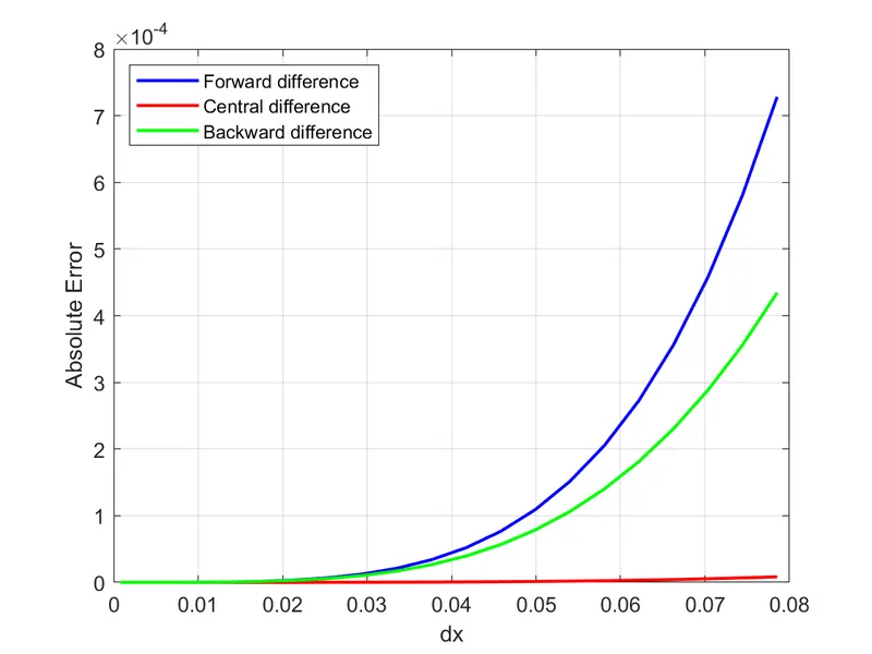
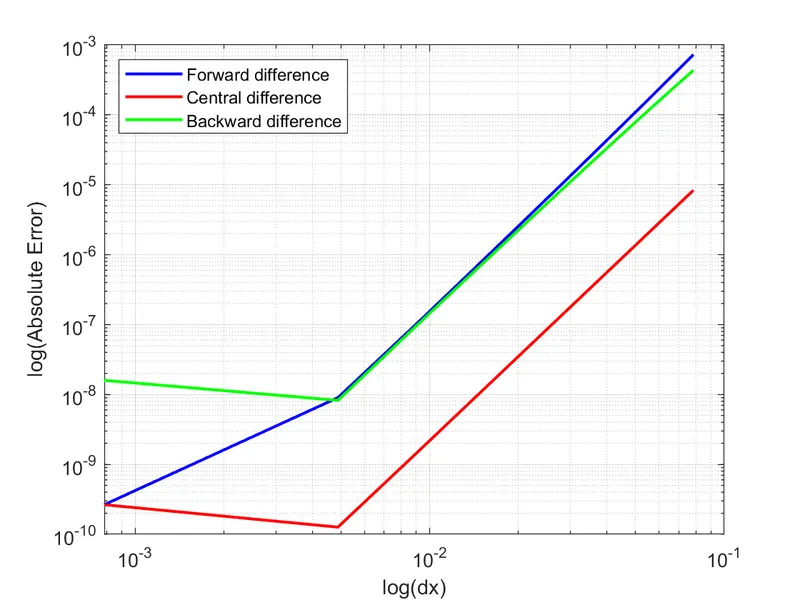
The error is minimum for Central Difference scheme as compared to Forward Difference and Backward Difference Schemes

The second plot shows forward difference error hold higher power relation compared with backward difference and central difference.

Conclusion:

As 'dx' size increases error also increases and vice versa. As confirmed from both the plots the error follows exponential relationship with the size of 'dx'.

We have seen from above plots that Central difference scheme is better than Forward Difference and Backward Difference Schemes in terms of accuracy. Central difference schemes are most accurate.

However, it requires the information of equal number of both forward and backward grid points which serves the purpose well for the points inside the domain, away from boundaries. But for grid points at the boundaries there is no information of either the backward or the forward grid point which leads to failure of Central Difference Scheme. In such cases Forward and Backward Difference Schemes are useful.