Project 2 - Rankine cycle Simulator

Aim:

1. Create a Rankine Cycle Simulator using MATLAB.
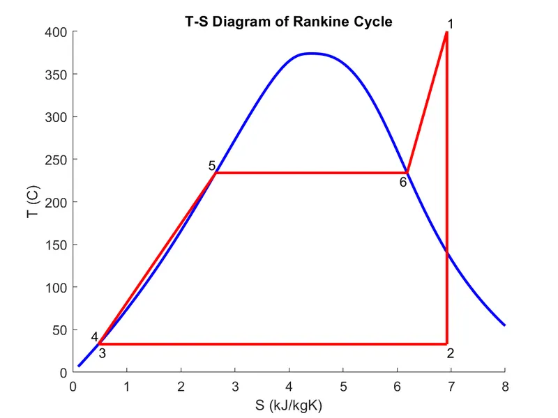
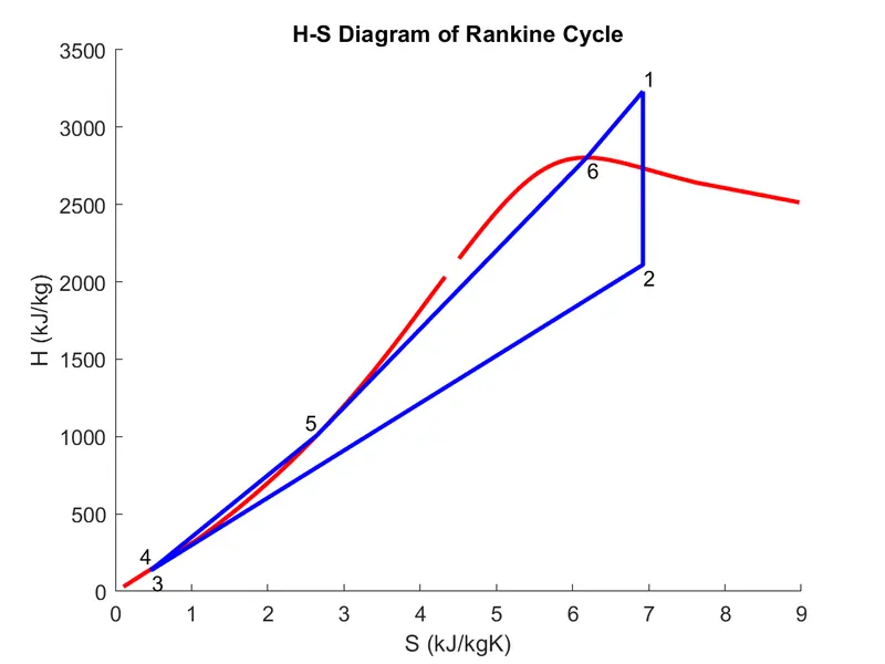
2. Then, plot the corresponding T-s and h-s plots for the given set of inputs.
3. Also calculate following parameters:
   1. Specific Steam Consumption
   2. Back Work Ratio

Theory:

Rankine cycle is a vapour power cycle with water as a working fluid.

It consists of 4 processes occuring in 4 components:

1. Isentropic expansion process occuring in the Turbine.
   1. The working fluid in form of steam enters the turbine and exit the turbine as wet or dry steam. It is highly recommended for steam to be on dryer side to prevent corrosion of turbine blades.
   2. Since entropy remains constant for the overall process, hence called isentropic process.
   3. The pressure drops from boiler pressure at turbine inlet to condenser pressure at turbine outlet.
   4. It is a work extraction process and is given by difference in the enthalpy of the working fluid at the inlet and the exit of the turbine i.e. W_t=(h1-h2).
2. Isobaric heat rejection process occuring in the Condenser.
   1. The wet/dry steam from turbine outlet is condensed to saturated liquid in condensor which acts as inlet for the feeding pump.
   2. Since phase change occurs for steam to water during the whole process the process apart from being isobaric is also isothermal.
   3. Heat is rejected to the atmosphere or the feed water to raise its temperature before feeding and is given by the difference between the enthalpy of the working fluid at the inlet and the exit of the condenser i.e. Q_rej=(h3-h2).
3. Isentropic compression process in the Pump.
   1. The working fluid is in subcooled region.
   2. Since the water has low compressibility, as the pressure rises from condenser pressure to boiler pressure, the change in specific volume of the fluid is insignificant.
   3. Since entropy remains constant for the overall process, hence called isentropic process.
   4. Work is done in driving the pump which can be calculated by the difference in the enthalpy of the working fluid at the inlet and the exit of the pump i.e.W_p= (h1-h2).
4. Isobaric heat addition process in the Boiler.
   1. The compressed water is fed to the boiler where the heat is supplied to it to raise its temperature before sending it to the turbine.
   2. The water goes from subcooled region to wet steam and then to superheat region during this process.
   3. The process occurs at constant pressure hence called isobaric process.
   4. Heat added is given by Q_add=(h1-h4).

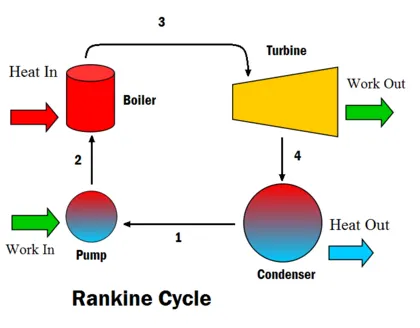
The whole cycle can be summed up by using following diagram:

Code:

The code is divided into 4 code sections:

1. First section extracts property values for various state of the rankine cycle.

p1=30;                       %turbine inlet pressure.
p2=0.05;
p3=p2;                       %pump inlet pressure.
p4=p1;                       %pump outlet pressure.
p5=p1;                       
p6=p1;                       %boiler outlet pressure.

T1=400;                      %temperature of working fluid at turbine inlet.
s1=XSteam('s_pT',p1,T1);     %entropy of working fluid at the turbine inlet.

s2=s1;                       %entropy of working fluid at turbine outlet.
s2f=XSteam('sL_p',p2);       %entropy of working fluid at saturated liquid state at turbine outlet pressure.
s2g=XSteam('sV_p',p2);       %entropy of working fluid at saturated vapour state at turbine outlet pressure.
s2fg=s2g-s2f;
x2=(s2-s2f)/s2fg;            %dryness fraction at the turbine outlet.

T2=XSteam('T_ps',p2,s2);     %temperature of working fluid at turbine outlet and condenser inlet.
T3=XSteam('TSat_p',p3);      %temperature at condenser outlet. since heat rejection is an isothermal process.
s3=XSteam('sL_T',T3);        %entropy of working fluid at the outlet of condenser and inlet of pump.
s4=s3;
T4=XSteam('T_ps',30,s3);     %temperature of working fluid at the outlet of the pump and the inlet of boiler.
T5=XSteam('TSat_p',p5);      %saturated liquid temperature of working fluid at boiler inlet pressure. 
s5=XSteam('sL_p',p5);
s6=XSteam('sV_p',p6);
T6=T5;                       %saturated vapour temperature of working fluid at boiler inlet pressure. 

h1=XSteam('h_pt',p1,T1);     %enthalpy of the working fluid at turbine inlet.

h2f=XSteam('hL_p',p2);
h2g=XSteam('hV_p',p2);
h2fg=h2g-h2f;
h2=h2f+x2*h2fg;              %enthalpy of the working fluid at turbne outlet.

h3=XSteam('hL_p',p3);        %enthalpy of the working fluid at the condenser outlet.
h4=XSteam('h_ps',p4,s4);     %enthalpy of the working fluid at the pump outlet.
h5=XSteam('hL_p',p5);        %enthalpy of saturated liquid phase of working fluid at boiler pressure.
h6=XSteam('hV_p',p6);        %enthalpy of saturated vapour phase of working fluid at the boiler pressure.

cp1=XSteam('Cp_pt',p1,T1);   %assuming cp1 as specific heat capacity for whole isentropic expansion process in turbine.
cp3=XSteam('CpL_p',p3);      %assuming cp3 as specific heat capacity for whole isentropic flow process in pump.
cp4=(h5-h4)/(T5-T4);         %specific heat coefficient for working fluid at pump outlet and boiler input.
cp5=XSteam('CpL_p',p5);      %specific heat coefficient for working fluid in boiler at saturated liquid phase. 

2. Sceond code section dispays these values in organized way.

%displaying state points and properties of working fluid at state points.
fprintf('-------------- Rankine Cycle Simulator ---------------\n\n');
disp('1-2 is Isentropic expansion process in turbine')
disp('2-3 is isobaric heat rejection process in condensor')
disp('3-4 is Isentropic compression process in pump')
disp('4-5-6 is isobaric heat addition process in boiler')

fprintf('\nThe pressure at turbine inlet (in bar): %3.0f',p1);
fprintf('\nThe temperature at turbine inlet (in °C): %3.0f',T1);
fprintf('\nThe pressure at turbine outlet (in bar): %3.2f\n\n',p2);

disp('--------------- RESULTS ---------------');

fprintf('\n\nState 1 properties:')
fprintf('\nP1 is: %3.0f bar\nT1 is: %3.0f °C\nh1 is: %3.0f kJ/kg\ns1 is: %f kJ/kgK',p1,T1,h1,s1)
fprintf('\n\nState 2 properties:')
fprintf('\nP2 is: %3.2f bar\nT2 is: %3.0f °C\nh2 is: %3.0f kJ/kg\ns2 is: %f kJ/kgK\ndryness fraction is: %f',p2,T2,h2,s2,x2)
fprintf('\n\nState 3 properties:')
fprintf('\nP3 is: %3.2f bar\nT3 is: %3.0f °C\nh3 is: %3.0f kJ/kg\ns3 is: %f kJ/kgK',p3,T3,h3,s3)
fprintf('\n\nState 4 properties:')
fprintf('\nP4 is: %3.0f bar\nT4 is: %3.0f °C\nh4 is: %3.0f kJ/kg\ns4 is: %f kJ/kgK',p4,T4,h4,s4)

fprintf('\n\nTurbine work is: %f kJ/kg',WT);
fprintf('\nPump work is: %f kJ/kg',WP);
fprintf('\nNet work is: %f kJ/kg',Wnet);
fprintf('\nHeat addition is: %f kJ/kg',QA);
fprintf('\nHeat rejection is: %f kJ/kg',QR);
fprintf('\nEfficiency of the cycle is: %f%%',eff);
fprintf('\nBack work ratio is: %f',bwr);
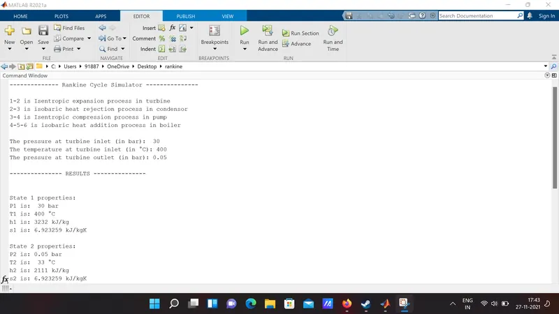
fprintf('\nSpecific Steam Consumption is: %f kg/kWhr',SSC);

The ouput in the command window:

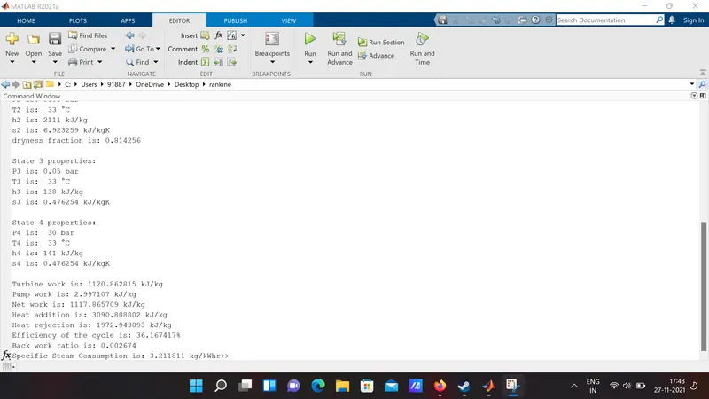
3. Third code section plots the T-S curve for a rankine cycle for given input parameters and calculates following parametes:

1. turbine work
2. pump work
3. net work
4. heat rejection
5. heat addition
6. back work ratio
7. specific steam consumption

%ploting saturation curve
figure(1)
S1=linspace(0.1,8,800);
for i=1:length(S1)
    T(i)=XSteam('TSat_s',S1(i));  %plotting saturation temperatures for all specific entropy values from 0.1 to 8.
end
hold on
plot(S1,T,'color','b','LineWidth',2);
    
%isentropic expansion in turbine
%entropy will remain the same for the process 
%the work done will be equal to drop in the enthalpy of the process
WT=h1-h2;                    %turbine work in kJ/kg

T_expansion=[T1 T2];        
s_expansion=[s1 s2];         %entropy remains same for the whole isentropic expaansion process. 

hold on
plot(s_expansion,T_expansion,'color','r','linewidth',2)
text(s1,T1,'1','VerticalAlignment','bottom');
xlabel('S (kJ/kgK)') ;
ylabel('T (C)');
title('T-S Diagram of Rankine Cycle');

%heat rejection process at constant pressure and temperature.
%this is possible due to whole process occurs during phase change of the working fluid.
%the latent heat of vapourization is rejected.
QR=h2-h3;
s_rejection=[s2 s3]; 
T_rejection=[T2 T3];         %isothermal and isobaric as phase change occurs.
plot(s_rejection,T_rejection,'color','r','linewidth',2)
text(s2,T2,'2','VerticalAlignment','top','HorizontalAlignment','left');

%pumping fluid to bolier at boiler inlet pressure
%this is an isentropic process
WP=h4-h3;
T_feed=[T3 T4];
s_feed=[s3 s4];
plot(s_feed,T_feed,'color','r','linewidth',2)
text(s3,T3,'3','VerticalAlignment','top');

%isobaric heat addition in boiler
QA=h1-h4;
s_heating=[s4,s5,s6,s1];
T_heating=[T4,T5,T6,T1];
plot(s_heating,T_heating,'color','r','linewidth',2);
text(s4,T4,'4','VerticalAlignment','bottom','HorizontalAlignment','right');
text(s5,T5,'5','VerticalAlignment','bottom','HorizontalAlignment','right');
text(s6,T6,'6','VerticalAlignment','top','HorizontalAlignment','right');

Wnet=WT-WP;
eff=(Wnet/QA)*100;
bwr=WP/WT;
SSC=3600/WT;

4.Fourth code section plots the H-S curve for a rankine cycle for given input parameters.

%plotting saturated enthalpy-entropy curve
figure(2)
P1=linspace(0.01,222,500);   %Since critical pressure of water is 221.2 bar  
for i=1:length(P1)
    SL(i)=XSteam('sL_p',P1(i));
    SV(i)=XSteam('sV_p',P1(i));
    HL(i)=XSteam('hL_p',P1(i));
    HV(i)=XSteam('hV_p',P1(i));
end
hold on
plot(SL,HL,'color','r','LineWidth',2);
plot(SV,HV,'color','r','LineWidth',2);
xlabel('S (kJ/kgK)');
ylabel('H (kJ/kg)');
title('H-S Diagram of Rankine Cycle');

%plotting enthalpy-entropy curve of whole cycle
H=[h1 h2 h3 h4 h5 h6 h1];
S=[s1 s2 s3 s4 s5 s6 s1];
plot(S,H,'color','b','linewidth',2);
text(s1,h1,'1','VerticalAlignment','bottom');
text(s2,h2,'2','VerticalAlignment','top','HorizontalAlignment','left');
text(s3,h3,'3','VerticalAlignment','top');
text(s4,h4,'4','VerticalAlignment','bottom','HorizontalAlignment','right');
text(s5,h5,'5','VerticalAlignment','bottom','HorizontalAlignment','right');
text(s6,h6,'6','VerticalAlignment','top');

T-S and H-S plots: