Week 9 - FVM Literature Review
Objective : To describe (a) Finite Volume Method (FVM).(b)major differences between FDM & FVM,(c)need for interpolation schemes and flux limiters in FVM.
Concept:
In computational fluid dynamics (CFD) there are 3 commonly used numerical method based solvers to solve the governing equations i.e Navier Stokes
Equations. These 3 methods are:
1.Finite Difference Method :
i.Finite-difference methods (FDM) are discritizations used for solving differential equations by approximating them with difference equations that finite
differences approximate the derivatives.
ii.FDMs convert a linear ordinary differential equations (ODE) or non-linear partial differential equations (PDE) into a system of equations that can be solved by matrix algebra techniques. For FDMs the grid is linear and should be aligned in such a way that all grid points lie in a straight line. The properties and governing equations are considered to be concentrated at a single point.
iii.We cannot use FDM directly to a body whose grid points are not aligned correctly along the x, y or z directions. These situations may occur due to
complex designs, folds and cuts in an geometry.
Since it is not aligned we cannot calculate the properties at the next adjacent point exactly (since there is an inclination between 2 mesh points), but we
can use some correction factor in order to approximate the difference with that adjacent point. This Method is known as Variable Transformation Method.
This approach seeks to create a grid using other space variables such as eta and epsilon. These space grids looks similar to a cartesian grid. A suitable
mapping function is defined and this function can be easily transformed through cartesian to new space vaiables (eta,epsilon) and vice versa.
The Variable Transformation Method gives an approximate solution of the property and also time consuming and complex.
For complex profiles and moving parts the above method is less preferred.
Due to this Finite Volume Method (FVM) is used.
2.Finite Volume Method :
i.The finite volume method (FVM) is a method for representing and evaluating partial differential equations PDEs in the form of algebraic equations. In the finite
volume method, volume integrals in a partial differential equation that contain a divergence term are converted to surface integrals, using the divergence
theorem. These terms are then evaluated as fluxes at the surfaces of each finite volume. Because the flux entering a given volume is identical to that leaving the
adjacent volume, these methods are conservative. Another advantage of the finite volume method is that it is easily formulated to allow for unstructured
meshes. The method is used in many computational fluid dynamics packages. "Finite volume" refers to the small volume surrounding each node point on a
mesh.
ii.Th method is applied over a volume so that the governing equation is valid over the entire volume. The properties are assumed to be concentrated at the
centre area. The volume integrals in a partial differential equation containing a divergence term are converted into surface integrals, using the divergence
theorem. The obtained terms are considered as fluxes at the surfaces of each finite volume because when we look through these discretised equations the flux
entering a given volume is identical to that leaving the adjacent volume, which is known as conservative. FVM is widely used as it can be applied for complex
geometry and moving parts.
ii.The finite volume method (FVM) is a method for representing and evaluating partial differential equations PDEs in the form of algebraic equations. In the finite
volume method, volume integrals in a partial differential equation that contain a divergence term are converted to surface integrals, using the divergence
theorem. These terms are then evaluated as fluxes at the surfaces of each finite volume. Because the flux entering a given volume is identical to that leaving the
adjacent volume, these methods are conservative. Another advantage of the finite volume method is that it is easily formulated to allow for unstructured
meshes. The method is used in many computational fluid dynamics packages. "Finite volume" refers to the small volume surrounding each node point on a
mesh.
3.Finite Element Method :
The FEM is a particular numerical method for solving PDEs in two or three space variables. For solving a problem, the FEM subdivides a large system into
smaller, simpler parts that are called finite elements. The finite element method finally results in a system of algebraic equations. This method approximates
the unknown function over the domain. The simple equations that model these finite elements are then assembled into a larger system of equations that
models the entire problem.
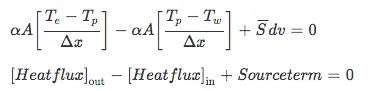
Consider a steady state heat conduction equation with a source term (heat generation source) :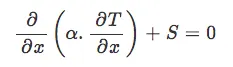 .....................(1)
where
S = the Source term.
`alpha`=thermal diffusivity term.
`(delT)/(delx)`=Temperature gradient along x direction.
The above governing equation is valid at every point in the domain, meaning it is valid for the entire control volume.
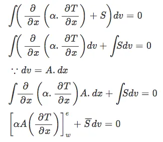
If we consider a small control volume (dv) and it is multiplied with the governing equation and integrated for entire volume then that should also be equal to
zero i.e. the integral form of governing equation.
Taking the conservation equation validated at single point and if it is validated at single point then it is validated atentire volume and in this entire volume the
properties are conserved.
Multiplying the equation by 'dv' and integrating it, we obtain
 ..................(2)
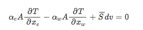 ..........................(3)
If we assume as a constant and not as a function of temperature,
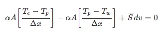 .................(4)
The source term which is to be added in a cell, if it is a function of temperature we have to linearize it. If we consider as a function of temperature we have to
linearize it as well.
 .............(5)
Interpolation Scheme :
In the finite volume formulation, evaluation of surface and volume integrals sometimes requires the values of unknown variables at locations other than the
computational nodes of the control volume. These values are obtained by employing certain interpolation schemes.
As an example let us consider the simple case of steady state one dimensional convection and diffusion.
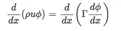 ........................................(6)
`phi`=solution variable (scalar)
`rho`=density
`u`=velocity
Integration of the governing differential equation over the control volume around grid point P yeilds:
 .................(7)
Some interpolation schemes used in CFD are as follows:
1. Upwind interpolation scheme.
2. Linear interpolation scheme.
3. Quadratic Upwind interpolation for convective Kinematics (QUICK) scheme.
4. Hybrid Scheme.
5. Total Variation Diminishing (TVD) scheme.
FLUX LIMITERS:
1.Flux limiters are used in the numerical schemes to solve problems of fluid dynamics, described by highly coupled non-linear Partial Differential Equations. If we tend to use low order numerical schemes for the solving of the governing equations then we might get a highly oscillatory and unstable solution near the discontinuity if present. Whereas if we tend to use higher-order numerical schemes to capture the phenomenon more accurately we tend to exploit the computational power unnecessarily.
2.The main idea behind the use of the flux limiters is to limit the spatial derivative terms near the discontinuities to physical real values so as to maintain physical consistency. There are several types of flux/slope limiter functions. They come in handy when sharp wave-fronts/peaks
are present.
3.For smoothly changing waves/functions, the flux limiters do not operate and the spatial derivatives can be represented normally.
4.It is imperative to note that flux limiters are also referred to as slope limiters because they both have the same mathematical form, and both have the effect of
limiting the solution gradient near shocks or discontinuities.
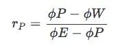
Flux limiter function depends upon the smoothness parameter r which is defined as:
 .........................................(8)
5.The flux limiter function is constrained to be greater than or equal to zero. It assumes a value of 0 near discontinuities anda value of 1 away from them. Hence it
switches between higher order scheme and lower order scheme for numerical representation of flux, thereby keeping the scheme stable and accurate
throughout.
6.The flux limiters are also referred to as slope limiters because they both have the same mathematical form, and both have the effect of limiting the solution
gradient near shocks or discontinuities. In general, the term flux limiter is used when the limiter acts on system fluxes and slope limiter is used when the limiter
acts on system states (like pressure and velocity).
7.If limiter function = 0, then there will be a low resolution and sharp gradient.
if limiter function > 0, then there will be a high resolution and positive gradient.