Week 7 - Simulation of a 1D Super-sonic nozzle flow simulation using Macormack Method
Aim: Simulating quasi 1-D supersonic flow through a converging diverging nozzle using MacCormack method
Objective:
Deducing the conservative and non-conservative forms of governing equations and implementing MacCormack method to solve the equations and
comparing the results.
Computing the steady state distribution of fluid variables in the nozzle and the time variation of the variables.
Studying the variation of mass flow rate inside the nozzle at different time steps under influence of time marching.
MATLABCODE
close all
clc
% Initializing the domain
L = 3;
nx = 21;
x = linspace(0,L,nx)';
dx = x(2)-x(1);
C = 0.2;
nt = 1100;
gamma = 1.4;
% Nozzle area profile
A = 1 + 2.2*(x-1.5).^2;
% Computing the flow variable through conservative and non-conservative form
[rho1, V1, T1, p1, M1, m1, rho_t1, V_t1, p_t1, T_t1, M_t1, residual1] = nonconservative(x, dx, A, C, nt,gamma);
[rho2, V2, T2, p2, M2, m2, rho_t2, V_t2, p_t2, T_t2, M_t2, residual2] = conservative(x, dx, A, C, nt, gamma);
% Plotting the results
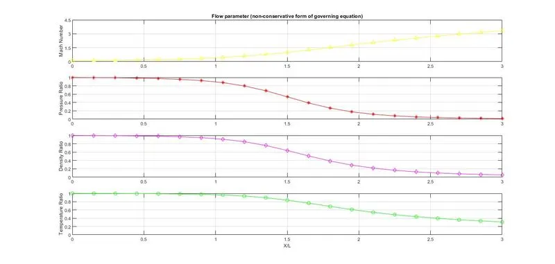
figure(1)
subplot(4,1,1)
plot(x,M1,'y^-')
grid on; ylim([0 4.5]); yticks(0:1.5:4.5);
ylabel('Mach Number')
title('Flow parameter (non-conservative form of governing equation)')
subplot(4,1,2)
plot(x,p1,'r*-')
grid on; yticks(0:0.2:1);
ylabel('Pressure Ratio')
subplot(4,1,3)
plot(x,rho1,'md-')
grid on; yticks(0:0.2:1);
ylabel('Density Ratio')
subplot(4,1,4)
plot(x,T1,'go-')
grid on; ylim([0 1]); yticks(0:0.2:1);
ylabel('Temperature Ratio')
xlabel('X/L')
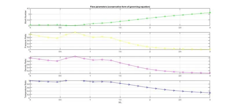
figure(2)
subplot(4,1,1)
plot(x,M2,'g*-')
grid on; ylim([0 4.5]); yticks(0:1.5:4.5);
ylabel('Mach Number')
title('Flow parameters (conservative form of governing equation)')
subplot(4,1,2)
plot(x,p2,'yd-')
grid on; yticks(0:0.2:1);
ylabel('Pressure Ratio')
subplot(4,1,3)
plot(x,rho2,'mo-')
grid on; yticks(0:0.2:1);
ylabel('Density Ratio')
subplot(4,1,4)
plot(x,T2,'b>-')
grid on; ylim([0 1]); yticks(0:0.2:1);
ylabel('Temperature Ratio')
xlabel('X/L')
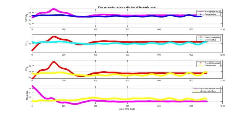
figure(3)
subplot(4,1,1)
plot(1:nt,rho_t1,'m^-')
hold on
plot(1:nt,rho_t2,'bp-')
grid on; ylim([0 1]); yticks(0:0.2:1);
ylabel('rho/rho_0')
title('Flow parameter variation with time at the nozzle throat');
legend('Non-conservative','Conservative');
subplot(4,1,2)
plot(1:nt,T_t1,'ro-')
hold on
plot(1:nt,T_t2,'c*-')
grid on; yticks(0:0.2:1);
ylabel('T/T_0')
legend('Non-conservative','Conservative');
subplot(4,1,3)
plot(1:nt,p_t1,'r*-')
hold on
plot(1:nt,p_t2,'yo-')
grid on; yticks(0:0.2:1);
ylabel('p/p_0')
legend('Non-conservative','Conservative')
subplot(4,1,4)
plot(1:nt,M_t1,'m>-')
hold on
plot(1:nt,M_t2,'y^-')
grid on; yticks(0:0.2:2);
ylabel('Mach No.')
xlabel('no.of time steps')
legend('Non-conservative form','Conservative form')
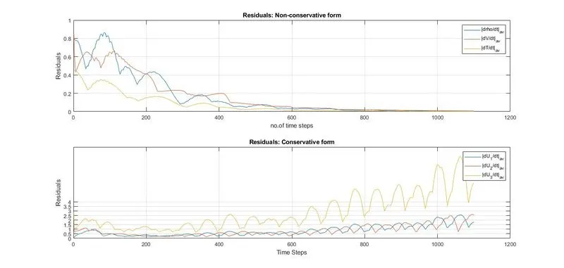
figure(4)
subplot(2,1,1)
plot(1:nt,residual1)
grid on
xlabel('no.of time steps')
ylabel('Residuals')
legend('|drho/dt|_{av}','|dV/dt|_{av}','|dT/dt|_{av}')
title('Residuals: Non-conservative form')
subplot(2,1,2)
plot(1:nt,residual2)
grid on
xlabel('Time Steps')
ylabel('Residuals'); yticks(0:0.5:4);
legend('|dU_1/dt|_{av}','|dU_2/dt|_{av}','|dU_3/dt|_{av}')
title('Residuals: Conservative form')
figure(5)
hold on; grid on;
plot(x,m1(50,:),'y')
plot(x,m1(100,:),'d')
plot(x,m1(150,:),'g')
plot(x,m1(200,:),'m')
plot(x,m1(700,:),'c')
xlabel('X/L')
ylabel('rhoAV/rho_0A_0V_0')
legend('t = 50/t','t = 100/t','t = 150/t','t = 200/t','t = 700/t')
title('Variation of non-dimensional mass flow rate (Non-conservative form)')
figure(6)
hold on; grid on;
plot(x,m2(100,:),'g')
plot(x,m2(150,:),'d')
plot(x,m2(200,:),'y')
plot(x,m2(700,:),'m')
xlabel('X/L')
ylabel('rhoAV/rho_0A_0V_0')
legend('t = 100/t','t = 150/t','t = 200/t','t = 700/t')
title('Variation of non-dimensional mass flow rate (Conservative form)')
figure(7)
hold on; grid on;
plot(x,m1(end,:))
plot(x,m2(end,:))
plot(x,0.579*ones(length(x),1),'-r*')
xlabel('X/L')
ylabel('rhoAV/rho_0A_0V_0')
legend('Non-conservative','Conservative','Exact')
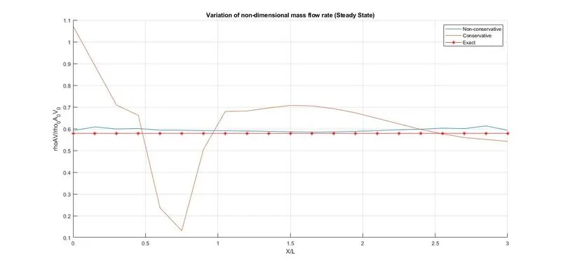
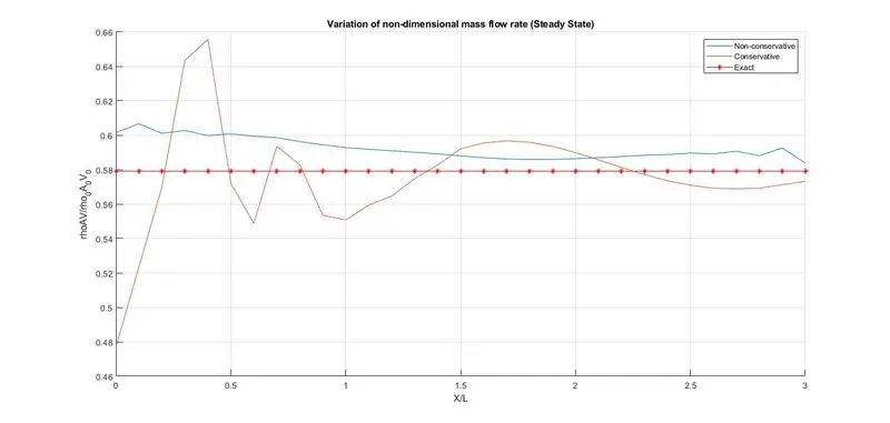
title('Variation of non-dimensional mass flow rate (Steady State)')
% Solver for Conservative Form of Governing Equation
function [rho, V, T, p, M, m, rho_t, V_t, p_t, T_t, M_t, residual] = conservative(x, dx, A, C, nt, gamma)
% Initial conditions
rho_0 = zeros(length(x),1);
T_0 = rho_0;
V_0 = T_0;
for i=1:length(x)
if x(i)>=0 && x(i)<0.5
rho_0(i) = 1;
T_0(i) = 1;
elseif x(i)>=0.5 && x(i)<1.5
rho_0(i) = 1 - 0.366*(x(i)-0.5);
T_0(i) = 1 - 0.167*(x(i)-0.5);
elseif x(i)>=1.5 && x(i)<=3
rho_0(i) = 0.634 - 0.3879*(x(i)-1.5);
T_0(i) = 0.833 - 0.3507*(x(i)-1.5);
end
V_0(i) = 0.59/(rho_0(i)*A(i));
end
throat = find(A==1);
rho = rho_0;
T = T_0;
V = V_0;
m = zeros(nt,length(x));
U1 = rho.*A;
U2 = rho.*A.*V;
U3 = rho.*(T./(gamma-1) + 0.5*gamma*V.^2).*A;
rho_t = zeros(nt,1);
T_t = rho_t;
V_t = T_t;
p_t = V_t;
M_t = p_t;
residual = zeros(nt,3);
for k=1:nt
U1_old = U1; U2_old = U2; U3_old = U3;
dt = min(C*dx./(T.^0.5 + V));
F1 = U2;
F2 = (U2.^2)./U1+((gamma-1)/gamma)*(U3 - 0.5*gamma*(U2.^2)./U1);
F3 = gamma*U2.*U3./U1 - 0.5*gamma*(gamma-1)*(U2.^3)./(U1.^2);
% Predictor loop
for i=2:length(x)-1
dF1dx = (F1(i+1) - F1(i))/dx;
dF2dx = (F2(i+1) - F2(i))/dx;
dF3dx = (F3(i+1) - F3(i))/dx;
dAdx = (A(i+1) - A(i))/dx;
J2 = (1/gamma)*rho(i)*T(i)*dAdx;
dU1dt_p(i) = -dF1dx;
dU2dt_p(i) = -dF2dx + J2;
dU3dt_p(i) = -dF3dx;
% Intermediate update
U1(i) = U1(i) + dU1dt_p(i)*dt;
U2(i) = U2(i) + dU2dt_p(i)*dt;
U3(i) = U3(i) + dU3dt_p(i)*dt;
end
rho = U1./A;
V = U2./U1;
T = (gamma-1)*((U3./U1) - 0.5*gamma*V.^2);
F1 = U2;
F2 = (U2.^2)./U1+((gamma-1)/gamma)*(U3 - 0.5*gamma*(U2.^2)./U1);
F3 = gamma*U2.*U3./U1 - 0.5*gamma*(gamma-1)*(U2.^3)./(U1.^2);
% Corrector loop
for i=2:length(x)-1
dF1dx = (F1(i) - F1(i-1))/dx;
dF2dx = (F2(i) - F2(i-1))/dx;
dF3dx = (F3(i) - F3(i-1))/dx;
dAdx = (A(i) - A(i-1))/dx;
J2 = (1/gamma)*rho(i)*T(i)*dAdx;
dU1dt_c(i) = -dF1dx;
dU2dt_c(i) = -dF2dx + J2;
dU3dt_c(i) = -dF3dx;
end
% Average of predictor and corrector step
dU1dt = 0.5*(dU1dt_p + dU1dt_c);
dU2dt = 0.5*(dU2dt_p + dU2dt_c);
dU3dt = 0.5*(dU3dt_p + dU3dt_c);
residual(k,1) = max(abs(dU1dt));
residual(k,2) = max(abs(dU2dt));
residual(k,3) = max(abs(dU3dt));
% Final solution update
for i=2:length(x)-1
U1(i) = U1_old(i) + dU1dt(i)*dt;
U2(i) = U2_old(i) + dU2dt(i)*dt;
U3(i) = U3_old(i) + dU3dt(i)*dt;
end
% Boundary conditions
U1(1) = rho(1)*A(1);
U1(end) = 2*U1(end-1) - U1(end-2);
U2(1) = 2*U2(2) - U2(3);
U2(end) = 2*U2(end-1) - U2(end-2);
U3(1) = U1(1)*((T(1)/(gamma-1)) + 0.5*gamma*V(1)^2);
U3(end) = 2*U3(end-1) - U3(end-2);
rho = U1./A;
V = U2./U1;
T = (gamma-1)*((U3./U1) - 0.5*gamma*V.^2);
M = V./(T.^0.5);
p = rho.*T;
m(k,:) = rho.*A.*V;
rho_t(k) = rho(throat); V_t(k) = V(throat); T_t(k) = T(throat);
p_t(k) = p(throat); M_t(k) = M(throat);
end
end
% Solver for Non-Conservative Form of Governing Equation
function [rho, V, T, p, M, m, rho_t, V_t, p_t, T_t, M_t, residual] = nonconservative(x, dx, A, C, nt, gamma)
% Initial conditions
rho_0 = 1 - 0.3146*x;
T_0 = 1 - 0.2314*x;
V_0 = (0.1 + 1.09*x).*T_0.^0.5;
throat = find(A==1);
rho = rho_0; T = T_0; V = V_0; m = zeros(nt,length(x));
rho_t = zeros(nt,1); T_t = rho_t; V_t = T_t; p_t = V_t; M_t = p_t;
residual = zeros(nt,3);
for k=1:nt
rho_old = rho; T_old = T; V_old = V;
dt = min(C*dx./(T.^0.5 + V));
% Predictor loop
for i=2:length(x)-1
dVdx = (V(i+1) - V(i))/dx;
dlogAdx = (log(A(i+1))-log(A(i)))/dx;
drhodx = (rho(i+1) - rho(i))/dx;
dTdx = (T(i+1) - T(i))/dx;
drhodt_p(i) = -rho(i)*dVdx - rho(i)*V(i)*dlogAdx - V(i)*drhodx;
dVdt_p(i) = -V(i)*dVdx - (1/gamma)*(dTdx + (T(i)/rho(i))*drhodx);
dTdt_p(i) = -V(i)*dTdx - (gamma-1)*T(i)*(dVdx + V(i)*dlogAdx);
% Intermediate update
rho(i) = rho(i) + drhodt_p(i)*dt;
V(i) = V(i) + dVdt_p(i)*dt;
T(i) = T(i) + dTdt_p(i)*dt;
end
% Corrector loop
for i=2:length(x)-1
dVdx = (V(i) - V(i-1))/dx;
dlogAdx = (log(A(i))-log(A(i-1)))/dx;
drhodx = (rho(i) - rho(i-1))/dx;
dTdx = (T(i) - T(i-1))/dx;
drhodt_c(i) = -rho(i)*dVdx - rho(i)*V(i)*dlogAdx - V(i)*drhodx;
dVdt_c(i) = -V(i)*dVdx - (1/gamma)*(dTdx + (T(i)/rho(i))*drhodx);
dTdt_c(i) = -V(i)*dTdx - (gamma-1)*T(i)*(dVdx + V(i)*dlogAdx);
end
% Average of predictor and corrector step
drhodt = 0.5*(drhodt_p + drhodt_c);
dVdt = 0.5*(dVdt_p + dVdt_c);
dTdt = 0.5*(dTdt_p + dTdt_c);
residual(k,1) = max(abs(drhodt));
residual(k,2) = max(abs(dVdt));
residual(k,3) = max(abs(dTdt));
% Final solution update
for i=2:length(x)-1
rho(i) = rho_old(i) + drhodt(i)*dt;
V(i) = V_old(i) + dVdt(i)*dt;
T(i) = T_old(i) + dTdt(i)*dt;
end
% Boundary conditionsno.of time steps
rho(end) = 2*rho(end-1)-rho(end-2);
V(1) = 2*V(2)-V(3); V(end) = 2*V(end-1)-V(end-2);
T(end) = 2*T(end-1)-T(end-2);
M = V./(T.^0.5);
p = rho.*T;
m(k,:) = rho.*A.*V;
rho_t(k) = rho(throat); V_t(k) = V(throat); T_t(k) = T(throat);
p_t(k) = p(throat); M_t(k) = M(throat);
end
end
PLOTS
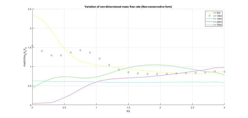
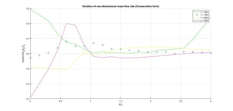
For n=21
For n=31
CONCLUSION
1.Conservative form is take less time as comapred to non conservative form as shown in the simulation data.
In grid dependence test we observe that the accuracy in case of non consevative form is more as comapared to conservative form as it is very close to
exact analytical solution.
2.In case of conservative and non-conservative form, the values of the flow variables at the throat of the nozzle are plotted at each time step. It
can be observed that at smller time-steps, the behaviour of non-conservative form shows unstable results. (it shows oscillations) but with increase in time step, the difference in conservative and non-conservative approach diminshes.
3.Residuals (average time derivatives of variables) of both the approaches the conservative form converges to a steady state faster than
non-conservative form.
4.Conservative form produces an almost constant mass flow rate but the non-conservative approach gave a highly fluctuating mass flow rate.
5.By increasing the grid size (nx), it is noted that the conservative form almost maintains its consistency but the non conservative form tends to become stable.
6.MaCormack method provides stable solutions near to exact solution of flow problems.