Week 5.1 - Mid term project - Solving the steady and unsteady 2D heat conduction problem

Aim:To solve the 2D heat conduction equation by using the point iterative techniques

Bounadry conditions:

Top Boundary = 600 K

Bottom Boundary = 900 K

Left Boundary = 400 K

Right Boundary = 800 K

Methods:

methods for solving implicit equations.

1. Jacobi

2. Gauss-seidel

3. Successive over-relaxation

absolute error criteria is 1e-4 or tolerance(tol)

1.MATLAB CODE for steady state analysis

clear all
close all
clc
% inputs
% number of grid points along x and y axis
nx= 20;
ny=20;
x=linspace(0,1,nx);
dx = x(2)-x(1);
y= linspace(0,1,ny);
z=fliplr(y);
f=1.1;
iter = 1;
t= 300*ones([nx,ny]);
% applying BC
t(1,:)=600;
t(end,:)=900;
t(:,1)=400;
t(:,end)=800;
% creating a copy
told=t;
r1=t;
error= 29;
tol = 1e-4;
for iterative_solver = 1:3;
while(error>tol);
for i=2:nx-1;
for j=2:ny-1;
if(iterative_solver==1);
t(i,j)= jacobi(t,told,i,j);
elseif(iterative_solver==2)
t(i,j)=GS(t,told,i,j);
elseif(iterative_solver==3)
t(i,j)= sor(t,told,i,j,f);
end
end
end
error = max(max(t-told));
told = t;
[u1,v1]=meshgrid(x,z);
% plot
if(iterative_solver==1);
figure(1);
contourf(u1,v1,t);
[C,h]= contourf(u1,v1,t);
colorbar;
colormap(jet);
clabel(C,h);
xlabel('x-axis');
ylabel('y-axis');
title_text=sprintf('jacobi iterantion number=%d',iter);
title(title_text);
pause(0.003);
elseif(iterative_solver==2);
figure(2);
contourf(u1,v1,t);
[C,h]= contourf(u1,v1,t);
colorbar;
colormap(jet);
clabel(C,h);
xlabel('x-axis');
ylabel('y-axis');
title_text=sprintf('GS iterantion number=%d',iter);
title(title_text);
pause(0.005);
else
    figure(3);
[C,h]= contourf(u1,v1,t);
colorbar;
colormap(jet);
clabel(C,h);
xlabel('x-axis');
ylabel('y-axis');
title_text=sprintf('sor iterantion number=%d',iter);
title(title_text);
pause(0.005);
end
iter=iter+1;
end
error=19;
iter=1;
t=r1;
told=t;
end
function out = jacobi(t,told,i,j)
out = 0.25*((told(i,j-1)+told(i,j+1)+told(i-1,j)+told(i+1,j)))
end
function out = GS(t,told,i,j)
out = 0.25*((t(i,j-1)+told(i,j+1)+t(i-1,j)+told(i+1,j)))
end
function out = sor(t,told,i,j,f)
out = (1-f)*told(i,j) + f*(0.25*(t(i,j-1)+told(i,j+1)+t(i-1,j)+told(i+1,j)))
end

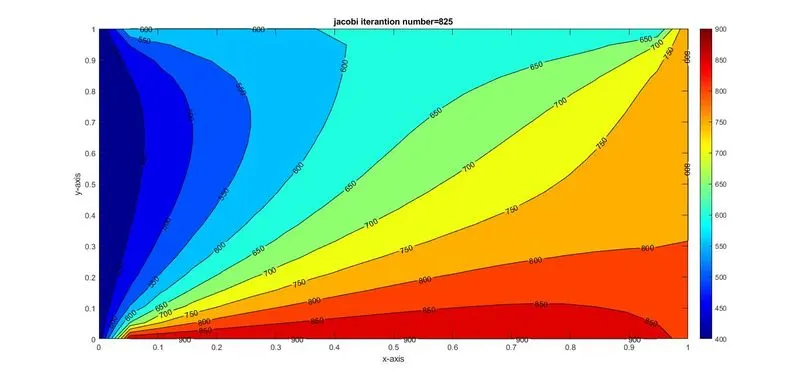
1.PLOT OF JCOBI ITERATION

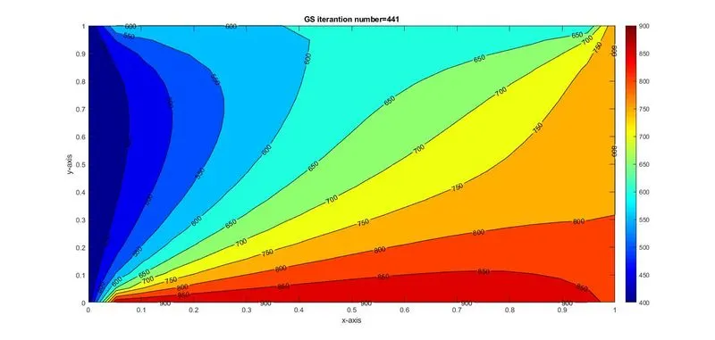
2.PLOT OF Gauss-seidel ITERATION

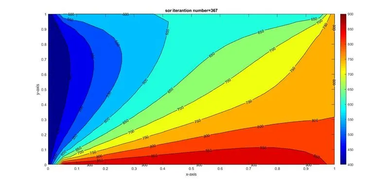
3.PLOT OF Successive over-relaxation ITERATION

conclusion

Successive over-relaxation iteration is the fastest among all the three iterations.And Jacobi iteration is the slowest among all three iterations.Gaus-Seidel act as in between and perform as moderate number of iterations.

2.MATLABCODE FOR UNSTEADY STATE OR Transient State Analysis

CASE-1 FOR EXPLICIT METHOD

clear all
close all
clc
% inputs
% number of grid points along x and y axis
nx= 10;
ny=10;
x=linspace(0,1,nx);
dx = x(2)-x(1);
y= linspace(0,1,ny);
dy = y(2)-y(1);
c= 1;
% number of steps
nt=200;
% time steps
dt = 0.001;
% CFL number
k= (c*dt)/dx^2;
t= ones([nx,ny])*673;
% applying BC
t(1,:)=600;
t(end,:)=900;
t(:,1)=400;
t(:,end)=800;
told = t;
tic
iter=1
for p=1:nt
for i= 2:nx-1
for j=2:ny-1
t(i,j)= k*(told(i-1,j)+told(i+1,j)+told(i,j+1)+told(i,j-1))+ (1-4*k)*told(i,j);
end
end
error=max(abs(told-t));
told=t;
iter=iter+1;
end
time = toc;
figure(1)
[c,h]=contourf(x,fliplr(y),t);
colorbar;
colormap(jet);
clabel(c,h);
title(sprintf('2D unsteady heat conduction (Explicit method) n iteration number=%d; t computational time:%0.4f',iter,time));
xlabel('xx');
ylabel('yy');

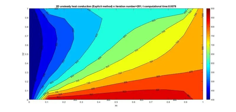
4.PLOT OF EXPLICIT METHOD OF UNSTEADY ANALYSIS

CASE-2 FOR IMPLICIT METHOD

clear all
close all
clc
% inputs
% number of grid points along x and y axis
nx= 20;
ny=20;
x=linspace(0,1,nx);
dx = x(2)-x(1);
y= linspace(0,1,ny);
dy = y(2)-y(1);
f= 1.2;
t= ones(nx,ny)*298;
% applying BC
t(1,:)=600;
t(end,:)=900;
t(:,1)=400;
t(:,end)=800;
alpha= 1.4;
dt=0.001;
% defining k1 and k2
k1=alpha*(dt/dx^2);
k2=alpha*(dt/dy^2);
told=t;
t_initial=t;
for iterartive_solver = 1:3
nt=1:1400;
error=9e9;
tol=1;
tic;
% iterartive_solver==1:3;
iter=1;
while error>tol
for i=2:nx-1
for j=2:ny-1
term1= 1/(1+2*k1+2*k2);
term2= k1*term1;
term3= k2*term1;
if iterartive_solver==1;
t(i,j)= ((told(i,j)*term1)+(term2*(t(i-1,j)+t(i+1,j))+(term3*(t(i,j-1)+t(i,j+1)))));
elseif iterartive_solver==2;
t(i,j)= ((told(i,j)*term1)+(term2*(t(i-1,j)+told(i+1,j))+(term3*(t(i,j-1)+told(i,j+1)))));
elseif iterartive_solver==3;
t(i,j)= (1-f)*told(i,j)+ f*(((told(i,j)*term1)+(term2*(t(i-1,j)+told(i+1,j))+(term3*(t(i,j-...
1)+told(i,j+1))))));
end
end
error_n=max(abs(told-t));
error=max(error_n);
told=t;
iter=iter+1;
end
end
time=toc;
%plot
if iterartive_solver==1;
figure(1)
contourf(x,fliplr(y),t);
[C,h]=contourf(x,fliplr(y),t);
colorbar;
colormap(jet);
clabel(C,h);
text = sprintf('JACOBI Method n iteration number = %d; t computational time: %0.4f',iter ,time);
title(text);
told=t_initial;
t=t_initial;
elseif iterartive_solver==2;
figure(2)
[c,h]=contourf(x,fliplr(y),t);
colorbar;
colormap(jet);
clabel(c,h);
title(sprintf('GS Method n iteration number = %d; t computational time: %0.4f',iter,time));
told=t_initial;
t=t_initial;
else
figure(3)
[c,h]=contourf(x,fliplr(y),t);
colorbar;
colormap(jet);
clabel(c,h);
title(sprintf('SOR Method n iteration number = %d; t computational time: %0.4f',iter,time));
told=t_initial;
t=t_initial;
end
end

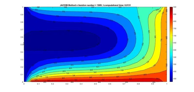
5.PLOT OF IMPLICIT JACOBI ITERATION

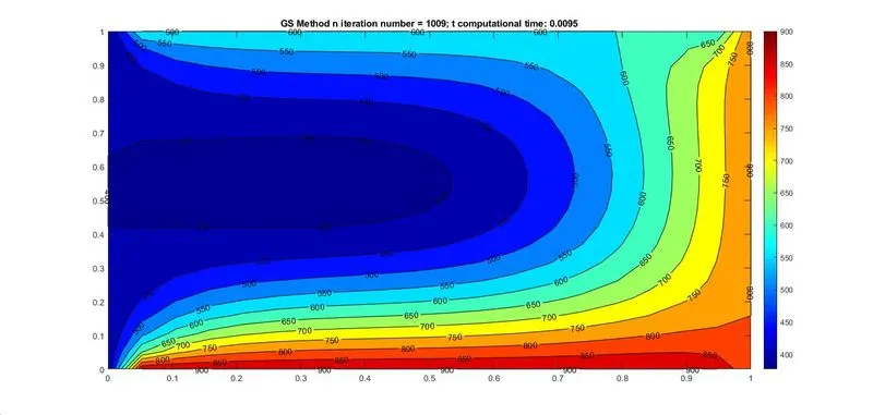
6.PLOT OF IMPLICIT Gauss-seidel ITERATION

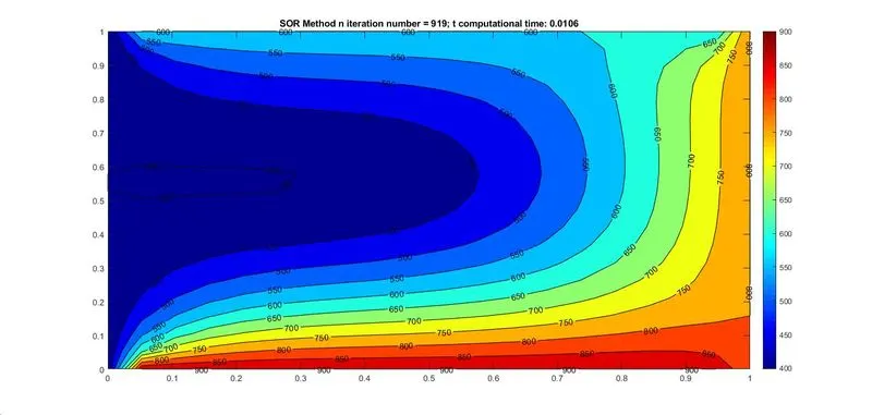
7.PLOT OF IMPLICIT Successive over-relaxation ITERATION

CONCLUSION

Implicit method will take hgher number of iteration as compared to explicit methds.And Successive over-relaxation iteration is the fastest and Jacobi itration is slowest and Gauss-Seidel method is act as an intermediate species among all.

Final conclusion

1Unsteady state iterative method will take more number of iteration as compared to Steady state methods.

2.Implict method is more accurate as compared to explicit method.