Week 9 - FVM Literature Review

Finite Volume Method (FVM):

The Finite Volume Method (FVM) is a type of discretization techniques used in Computational fluid dynamics which evaluates the partial differential equations into the algebraical form based on the control volume formulation. "Finite volume" refers to the small volume surrounding each node point on the mesh where variables are typically defined at the center of each control volume.

Steps Involved:

1. The first step in the FVM is to divide the domain into several control volumes where the variable of interest is located at the centroid of the control volume.
2. The next step is to integrate the differential form of the governing equations over each control volume using Gauss Divergence theorem. The resulting equation is called the discretized equation. In this manner, the discretization equation expresses the conservation principle for the variable inside the control volume.

• The most compelling feature of the FVM is that the resulting solution satisfies the conservation of quantities such as mass, momentum, energy, and species. This is exactly satisfied for any control volume as well as for the whole computational domain and for any number of control volumes. Even a coarse grid solution exhibits exact integral balances. It can be applied for complex geometry and moving parts.

Example: 1-D Linear heat conduction equation

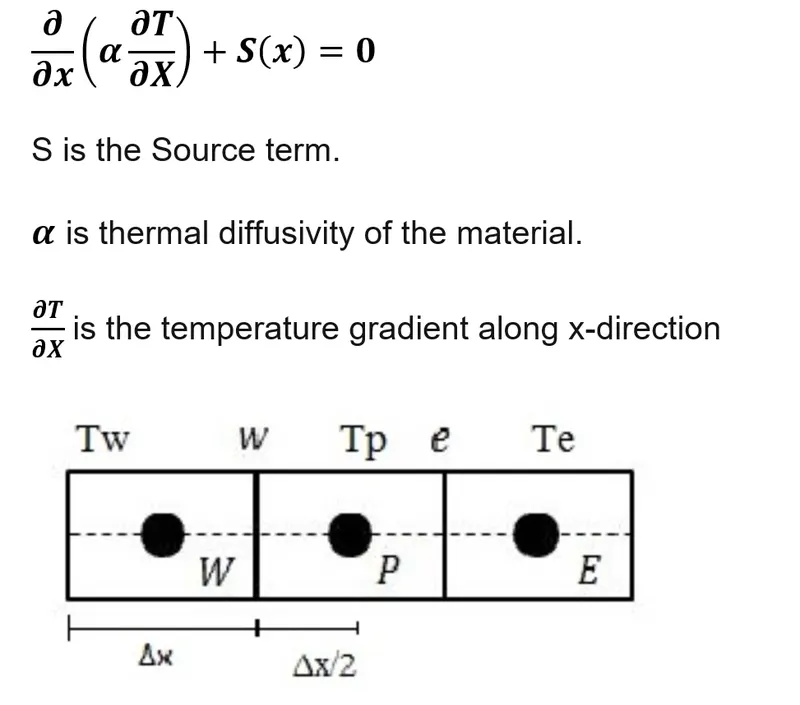
The above governing equation is valid at every point over the control volume. By following the Integration procedure mentioned above using Gauss Divergence theorem, we get the final equation as below

(Heat flux out) – (Heat flux in) + Source term = 0

The above terms specify that equation is conserved inside the domain.

Finite-difference methods (FDM)

FDM is a type of discretization technique that convert a linear ordinary differential equation and partial differential equation into a system of equations that can be solved using matrix algebra techniques. The grid is linear and should be aligned in such a way that all grid points lie in a straight line. So, we cannot calculate the properties at the next adjacent point exactly, but we can make some correction factor and approximations using 'Variable Transformation Method' which basically tries to create grid using different variable space which look very similar to cartesian grid. So, for complex geometries and curved faces, this method is not suited because the properties and governing equations are concentrated at a single point.

Interpolation Schemes:

Need:

If any results are to be computed other than the node points, with the help of values at the neighbor nodes, any of the approximation schemes is used. If the extreme two points are known, and if any value needs to compute in between then interpolation schemes are

In our case, to calculate the Tw and Te, we know the value at the T_P,T_E ,and T_W. So, using interpolation schemes, we can get the temperature at the east and west faces. Also, we can calculate thermal diffusivity of different faces.

Types:

1. Upwind interpolation scheme (UDS)
2. Linear interpolation scheme (CDS)
3. Quadratic Upwind Interpolation scheme (QUICK)
4. Hybrid Scheme

1. Upwind Interpolation scheme:

The upwind interpolation scheme (UDS) for approximating the value of a variable at either front or black face of a control volume is given by

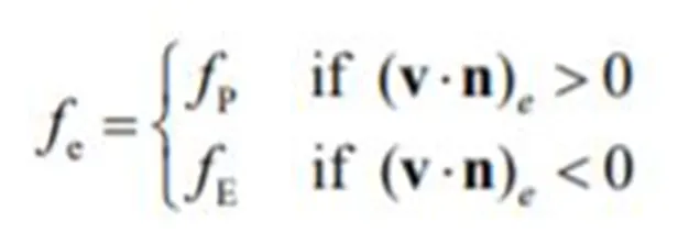
The interpolation scheme is equivalent to using a backward or forward finite difference approximation. It is the first order accurate scheme and is numerically diffusive with a coefficient of numerical diffusion

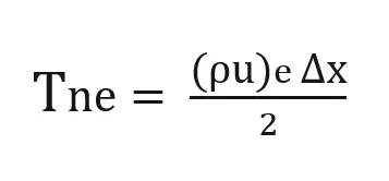
The scheme is developed from the convective flows with the suppressed diffusion effects.

2. Linear Interpolation scheme:

The value of the variable at CV face center approximates from the values near two computational nodes. This location at 'e' on a cartesian grid, the variable value is approximated by,

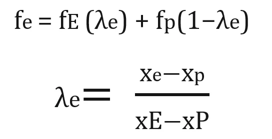
The linear interpolation is equivalent to the use of the central differencing formula of the first-order derivative, and hence, this is also termed as the central differencing scheme(CDS). This scheme is the second derivative accurate and may produce an oscillatory solution.

3. Quadratic Upwind interpolation(QUICK)

A quadratic upwind interpolation is the three-order scheme, it is derived from the polynomial fitting. It is also represented as the QUICK Interpolation. The quick interpolation on a uniform cartesian grid is given by,

ϕ_e=(6/8)*ϕ_U+(3/8)*ϕ_D-(1/8)ϕ_UU

Where D, U, and UU denote the downstream, the first upstream and the second upstream node respectively. (E, P, and W or P, E, and EE) depending on the flow direction. Quick scheme is prone to oscillation because of the third order.

4. Hybrid interpolation:

This companion of both the upwind and linear interpolation schemes. The cartesian grid is given by

Φf= ψΦ + (1−ψ) ⋅ Φcd

Where,

Φf = Value of the variable at the face(phi).

Φud = value of the variable at the face(by the upwind differencing technique).

Φcd = Value of the variable by Central differencing method at the face.

Ψ = blending function to switch between schemes.

Flux limiters:

While solving convective flow fields, discontinuity or shocks are observed in the solution. For the High order, instability is because the oscillations higher.

To obtain the highly accurate and oscillation free results, flux limiter functions are used. This function provides the smooth region over the flow and maintains the first-order accuracy.

Their simple forms for 1D Equation are given by

This terms represent edge fluxes for the i_th cell.

Where, fluxes can be represented by low and high-resolution schemes.

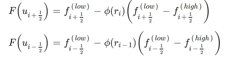
Where

f ^low=low resolution flux,

f ^high=high resolution flux,

ϕ(r)=flux limiter function.

where r represents the ratio of successive gradients on the solution mesh,

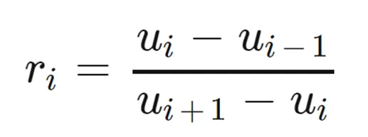
When the limiter equals to zero, the flux represents the low-resolution scheme.

When the limiter equals to 1, the flux represents the high-resolution scheme.

There are many limiters having distinguished characters and are selected according to the problem. There is no particular limiter found to work well for all and it is selected by the trial and error method.

Limiter types:

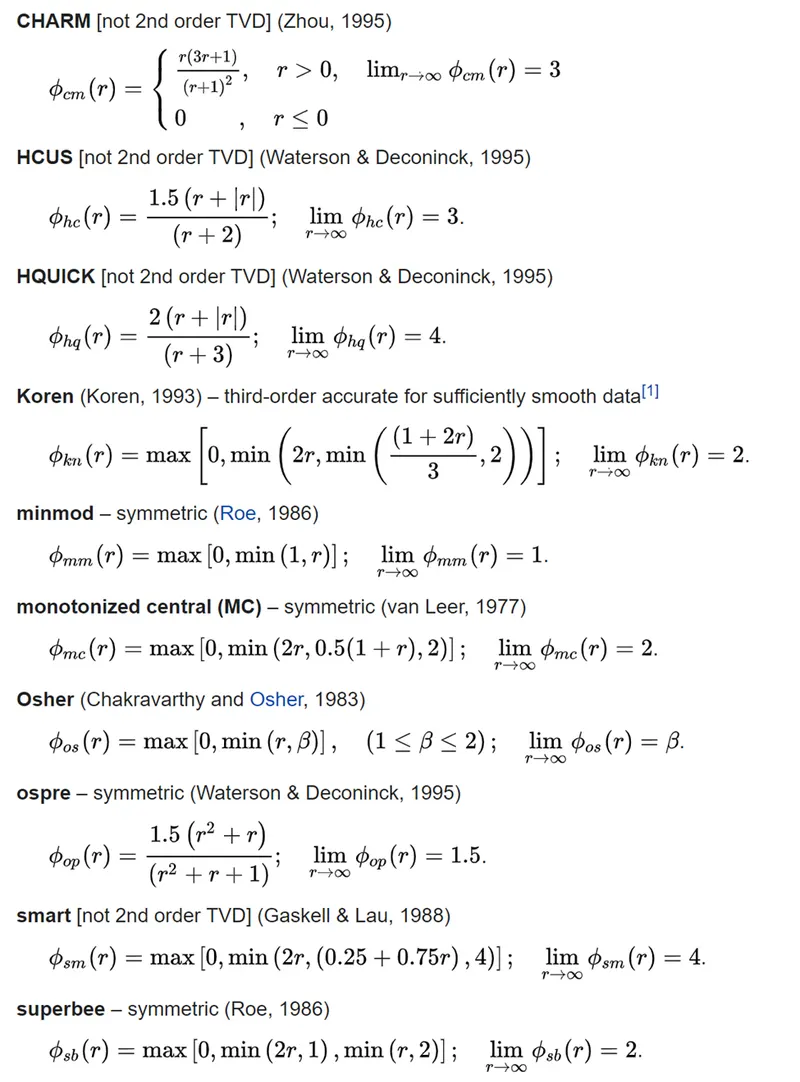
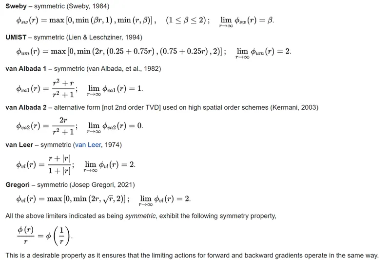
Note: Above content referred from Wikipedia