Week 5 - Mid term project - Solving the steady and unsteady 2D heat conduction problem
Equations
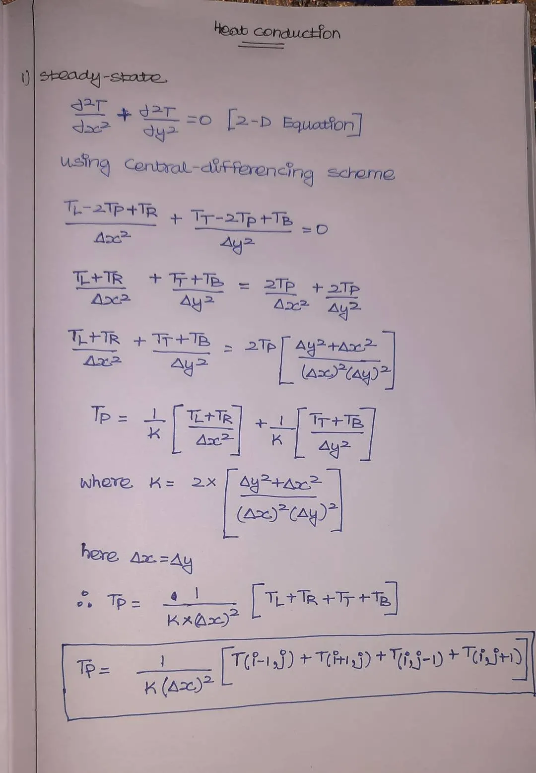
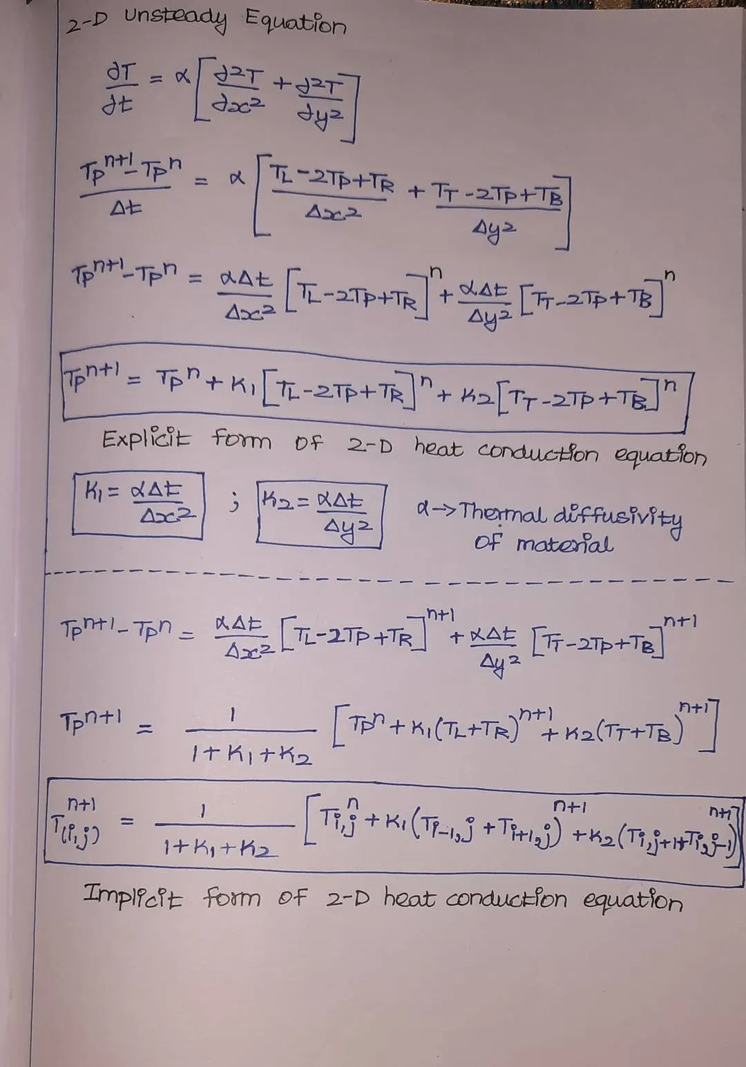
Coding:
1. The no. of meshpoints in the x and y direction are same (i.e 10). The x-domain and y-domain are divided into equal parts.
2. As per the given conditions, Temperature values are provided on the each sides of the domain. For the corner node, mean value between respective sides are taken.
3. The nodes which are free form boundary conditions are assigned with the temperature value of 300K
4. Then necessary error and tolerance values are assigned.
5. Since the problem has two subcategories,
(i) Steady state approach
(ii) Un-Steady state approach
6. To solve these equations different iterative solvers are used such as Jacobi, Gauss Seidel and Successive Over relaxation methods are used.
7. Necessary functions are created for different iterative solvers.
8. For the steady state approach, two space loops (x,y direction) are used to obtain the convergence and for the unsteady state approach , two space loops (x,y direction) and one time loop (time-derivative) are used to obtain the convergence.
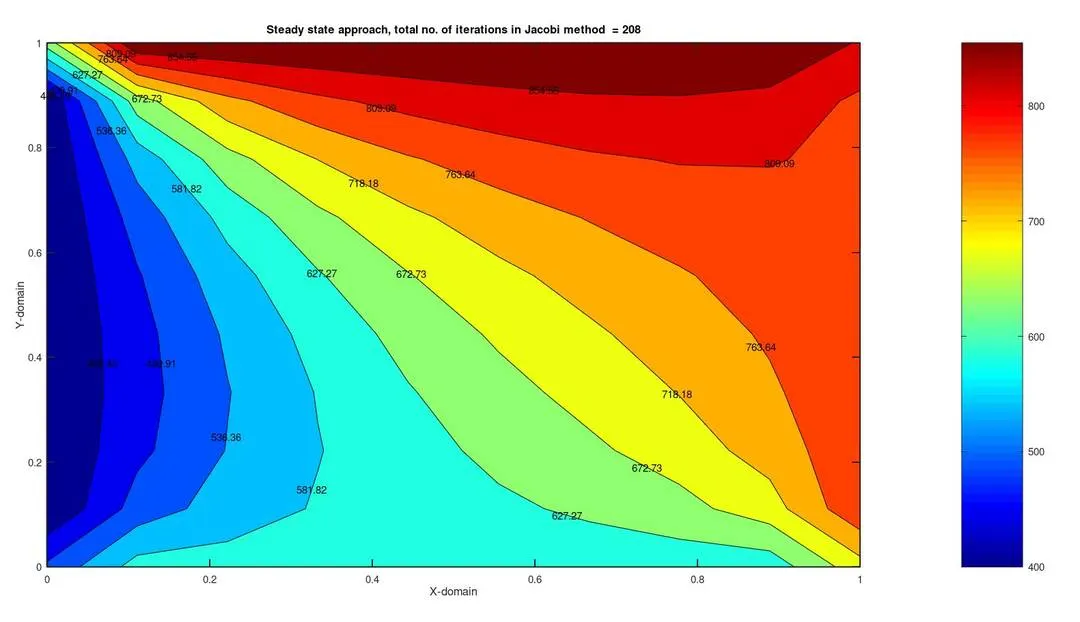
9. Finally to display the results,necessary graphs are plotted.
## Steady State Approach


## File no 1
## Main function


## steady state Approach

clear all
close all
clc

## Inputs

n_x=10;
n_y=10;
x=linspace(0,1,n_x);
y=linspace(0,1,n_y);
dx=x(3)-x(2);
dy=y(3)-y(2);

## Temperature values
T_t=600;
T_b=900;
T_l=400;
T_r=800;

t=300*(ones(n_x,n_y))


## Boundary conditions
t(1,1:n_x)=T_t;
t(n_y,1:n_x)=T_b;
t(2:n_y-1,1)=T_l;
t(2:n_y-1,n_x)=T_r;

## Modifying corner values
t(1,1)=(T_t+T_l)/2;
t(1,n_x)=(T_t+T_r)/2;
t(n_y,1)=(T_b+T_l)/2;
t(n_x,n_y)=(T_b+T_r)/2;

## Creating a copy of t
t_old=t
tolerance=1e-4;
error=9e9;

## K values
k=2*((dx^2+dy^2)/(dx^2*dy^2))

## Function call
jacobi_method=jacobi_steady_state(error,tolerance,n_x,n_y,t,t_old,dx,dy,x,y,k)
gauss_seidel_method=Gauss_seidel_steady_state(error,tolerance,n_x,n_y,t,t_old,dx,dy,x,y,k)
Sor_method=SOR_steady_state(error,tolerance,n_x,n_y,t,t_old,dx,dy,x,y,k)


## File no 2
## Jacobi_method

function value = jacobi_steady_state(error,tolerance,n_x,n_y,t,t_old,dx,dy,x,y,k)
jacobi_iteration=1
while(error>tolerance)
for i=2:n_x-1
 for j=2:n_y-1
    term1=(1/(k*dy^2))*(t_old(i,j-1)+t_old(i,j+1));
    term2=(1/(k*dx^2))*(t_old(i-1,j)+t_old(i+1,j));
    t(i,j)=term1+term2;
  endfor
endfor
error=max(max(abs(t_old-t)));
t_old=t;
jacobi_iteration=jacobi_iteration+1
endwhile

## plotting the graph
figure(1)
[c,d]=contourf(x,y,t)
clabel(c,d,'fontsize',15)
colormap(jet)
colorbar('fontsize',15)
title_text=sprintf('Steady state approach, total no. of iterations in Jacobi method  = %d',jacobi_iteration)
title(title_text)
set(gca,'fontsize',15,'linewidth',2)
xlabel('X-domain')
ylabel('Y-domain')
value=t
endfunction


## File no 3
## Gauss_seidel_method

function value = Gauss_seidel_steady_state(error,tolerance,n_x,n_y,t,t_old,dx,dy,x,y,k)

Gauss_seidel_iteration=1
while(error>tolerance)
for i=2:n_x-1
  for j=2:n_y-1
    t1=(t(i,j-1)+t_old(i,j+1))/(k*(dy^2));
    t2=(t(i-1,j)+t_old(i+1,j))/(k*(dx^2));
    t(i,j)=t1+t2;
  endfor
endfor
error=max(max(abs(t_old-t)));
t_old=t;
Gauss_seidel_iteration=Gauss_seidel_iteration+1
endwhile

## plotting the graph
figure(2)
[c,d]=contourf(x,y,t)
clabel(c,d,'fontsize',15)
colormap(jet)
colorbar('fontsize',15)
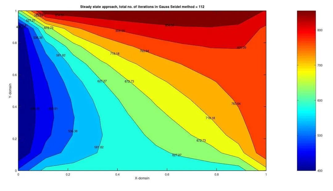
title_text=sprintf('Steady state approach, total no. of iterations in Gauss Seidel method = %d',Gauss_seidel_iteration)
title(title_text)
set(gca,'fontsize',15,'linewidth',2)
xlabel('X-domain')
ylabel('Y-domain')
value=t
endfunction


## File no 4
## SOR Method

function value = SOR_steady_state(error,tolerance,n_x,n_y,t,t_old,dx,dy,x,y,k)
omega=1.5;
SOR_iteration=1
while(error>tolerance)
for i=2:n_x-1
 for j=2:n_y-1
        t1=(1/(k*dy^2))*(t(i,j-1)+t_old(i,j+1));
        t2=(1/(k*dx^2))*(t(i-1,j)+t_old(i+1,j));
        temp=t1+t2;
        temp1=(omega)*(temp);
        temp2=(1-omega)*(t_old(i,j));
        t(i,j)=temp1+temp2;
  endfor
endfor
error=max(max(abs(t_old-t)));
t_old=t;
SOR_iteration=SOR_iteration+1
endwhile

## plotting the graph
figure(3)
[c,d]=contourf(x,y,t)
clabel(c,d,'fontsize',15)
colormap(jet)
colorbar('fontsize',15)
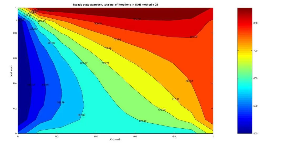
title_text=sprintf('Steady state approach, total no. of iterations in SOR method = %d',SOR_iteration)
title(title_text)
set(gca,'fontsize',15,'linewidth',2)
xlabel('X-domain')
ylabel('Y-domain')
value=t
endfunction
## File no 1
## Unsteady_Explicit_form
## Main Function

clear all
close all
clc

## Inputs

n_x=10;
n_y=10;
x=linspace(0,1,n_x);
y=linspace(0,1,n_y);
dx=x(2)-x(1);
dy=y(2)-y(1);
dt=0.0001
n_t=14000
alpha=1.4

## Temperature values
T_t=600;
T_b=900;
T_l=400;
T_r=800;

t=300*(ones(n_x,n_y))

## Boundary conditions
t(1,1:n_x)=T_t;
t(n_y,1:n_x)=T_b;
t(2:n_y-1,1)=T_l;
t(2:n_y-1,n_x)=T_r;

## Modifying corner values
t(1,1)=(T_t+T_l)/2;
t(1,n_x)=(T_t+T_r)/2;
t(n_y,1)=(T_b+T_l)/2;
t(n_x,n_y)=(T_b+T_r)/2;

## Creating a copy of t
t_old=t
tolerance=1e-4;
error=9e9;

## K values

k1=alpha*(dt/(dx^2))
k2=alpha*(dt/(dy^2))


Explicit_value=explicit_function(error,tolerance,n_x,n_y,t,t_old,dx,dy,x,y,k1,k2,dt,n_t)


## File no 2
## Unsteady_Explicit_function

function value=explicit_function(error,tolerance,n_x,n_y,t,t_old,dx,dy,x,y,k1,k2,dt,n_t)
iteration_no=1
while(error>tolerance)
  for i=2:n_x-1
    for j=2:n_y-1
      term_1 = t_old(i,j);
      term_2 = k1*((t_old(i+1,j) - 2*t_old(i,j) + t_old(i-1,j)));
      term_3 = k2*((t_old(i,j+1) - 2*t_old(i,j) + t_old(i,j-1)));
      t1=term_1+term_2+term_3;
      t(i,j)=t1;
    endfor
  endfor
  error=max(max(abs(t_old-t)))
  t_old=t;
  iteration_no=iteration_no+1

endwhile


## plotting the graph
figure(1)
[c,d]=contourf(x,y,t)
clabel(c,d,'fontsize',15)
colormap(jet)
colorbar('fontsize',15)
title_text=sprintf('Unsteady Explicit form, total no. of iterations in Explicit form  = %d',iteration_no)
title(title_text)
set(gca,'fontsize',15,'linewidth',2)
xlabel('X-domain')
ylabel('Y-domain')
value=t

endfunction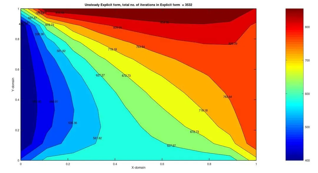
## Unsteady_state_approach
##Implicit_form

## File no 1
## Main_function


clear all
close all
clc

## Inputs

n_x=10;
n_y=10;
x=linspace(0,1,n_x);
y=linspace(0,1,n_y);
dx=x(2)-x(1);
dy=y(2)-y(1);
dt=2;
n_t=1400
alpha=1.4*e-5

## Temperature values
T_t=600;
T_b=900;
T_l=400;
T_r=800;

t=300*(ones(n_x,n_y))

## Boundary conditions
t(1,1:n_x)=T_t;
t(n_y,1:n_x)=T_b;
t(2:n_y-1,1)=T_l;
t(2:n_y-1,n_x)=T_r;

## Modifying corner values
t(1,1)=(T_t+T_l)/2;
t(1,n_x)=(T_t+T_r)/2;
t(n_y,1)=(T_b+T_l)/2;
t(n_x,n_y)=(T_b+T_r)/2;

## Creating a copy of t
t_old=t
t_prev=t
tolerance=1e-4;

## K values

k1=alpha*(dt/(dx^2))
k2=alpha*(dt/(dy^2))


## Function call

jacobi_method=jacobi_unsteady(tolerance,n_x,n_y,t,t_old,t_prev,dx,dy,x,y,k1,k2,dt,n_t)
gauss_seidel_method=Gauss_seidel_unsteady(tolerance,n_x,n_y,t,t_old,t_prev,dx,dy,x,y,k1,k2,dt,n_t)
Sor_method=SOR_unsteady(tolerance,n_x,n_y,t,t_old,t_prev,dx,dy,x,y,k1,k2,dt,n_t)


## File no 2
## Jacobi method function

function value = jacobi_unsteady(tolerance,n_x,n_y,t,t_old,t_prev,dx,dy,x,y,k1,k2,dt,n_t)
jacobi_iteration=1
time=0
for k=1:n_t
  error=9e9;
  while(error>tolerance)
  for i=2:n_x-1
   for j=2:n_y-1
      term_1 = (1+(2*k1)+(2*k2))^(-1);
      term_2 = k1*term_1;
      term_3 = k2*term_1;
      H = (t_old(i-1,j)+t_old(i+1,j));
      V = (t_old(i,j-1)+t_old(i,j+1));
      t(i,j)=(t_prev(i,j)*term_1)+(H*term_2)+(V*term_3);
    endfor
   endfor
  error=max(max(abs(t_old-t)))
  t_old=t;
  jacobi_iteration=jacobi_iteration+1
endwhile
conv = max(max(abs(t_prev-t)))
if conv<tolerance
  break
 end
 time = time+1
 t_prev=t;
endfor

## plotting the graph
figure(1)
[c,d]=contourf(x,y,t)
clabel(c,d,'fontsize',15)
colormap(jet)
colorbar('fontsize',15)
title_text=sprintf('Unsteady implicit form, Jacobi iteration value = %d',jacobi_iteration)
title(title_text)
set(gca,'fontsize',20,'linewidth',2)
xlabel('X-domain')
ylabel('Y-domain')

value=t
endfunction

## File no 3
## Gauss Seidel Method function

function value = Gauss_seidel_unsteady(tolerance,n_x,n_y,t,t_old,t_prev,dx,dy,x,y,k1,k2,dt,n_t)
Gauss_seidel_iteration=1
time = 0
for k=1:n_t
  error=9e9;
  while(error>tolerance)
   for i=2:n_x-1
    for j=2:n_y-1
      term_1 = (1+(2*k1)+(2*k2))^(-1);
      term_2 = k1*term_1;
      term_3 = k2*term_1;
      H = (t(i-1,j)+t_old(i+1,j));
      V = (t(i,j-1)+t_old(i,j+1));
      t(i,j)=(t_prev(i,j)*term_1)+(H*term_2)+(V*term_3);
    endfor
   endfor
  error=max(max(abs(t_old-t)))
  t_old=t;
  Gauss_seidel_iteration=Gauss_seidel_iteration+1
endwhile
conv = max(max(abs(t_prev-t)))
if conv<tolerance
  break
 end
 time = time+1
 t_prev=t;
endfor

## plotting the graph
figure(2)
[c,d]=contourf(x,y,t)
clabel(c,d,'fontsize',15)
colormap(jet)
colorbar('fontsize',15)
title_text=sprintf('Unsteady implicit form, Gauss Seidel iteration value = %d',Gauss_seidel_iteration)
title(title_text)
set(gca,'fontsize',20,'linewidth',2)
xlabel('X-domain')
ylabel('Y-domain')

value=t
endfunction


## File no 4
## SOR method function

function value = SOR_unsteady(tolerance,n_x,n_y,t,t_old,t_prev,dx,dy,x,y,k1,k2,dt,n_t)
SOR_iteration=1
omega=1.5;
time=0
for k=1:n_t
  error=9e9;
  while(error>tolerance)
  for i=2:n_x-1
   for j=2:n_y-1
      term_1 = 1/(1+(2*k1)+(2*k2));
      term_2 = k1*term_1;
      term_3 = k2*term_1;
      H = (t(i-1,j)+t_old(i+1,j));
      V = (t(i,j-1)+t_old(i,j+1));
      t(i,j)=omega*(t_prev(i,j)*term_1+(H*term_2)+(V*term_3))+(1-omega)*t_old(i,j);
   endfor
  endfor
  error=max(max(abs(t_old-t)))
  t_old=t;
  SOR_iteration=SOR_iteration+1
endwhile
conv = max(max(abs(t_prev-t)))
if conv<tolerance
  break
 end
 time = time+1
 t_prev=t;
endfor

## plotting the graph
figure(3)
[c,d]=contourf(x,y,t);
clabel(c,d,'fontsize',15);
colormap(jet);
colorbar('fontsize',15);
title_text=sprintf('Unsteady implicit form ,SOR iteration value = %d',SOR_iteration);
title(title_text);
set(gca,'fontsize',20,'linewidth',2);
xlabel('X-domain');
ylabel('Y-domain');

value=t
endfunction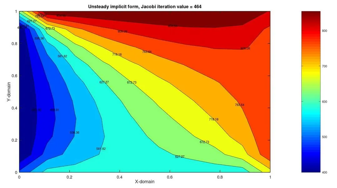
Results
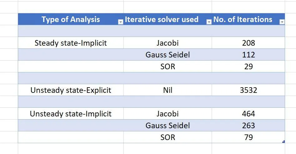
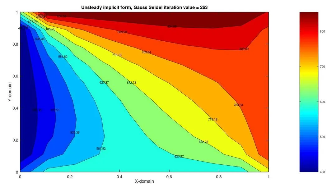
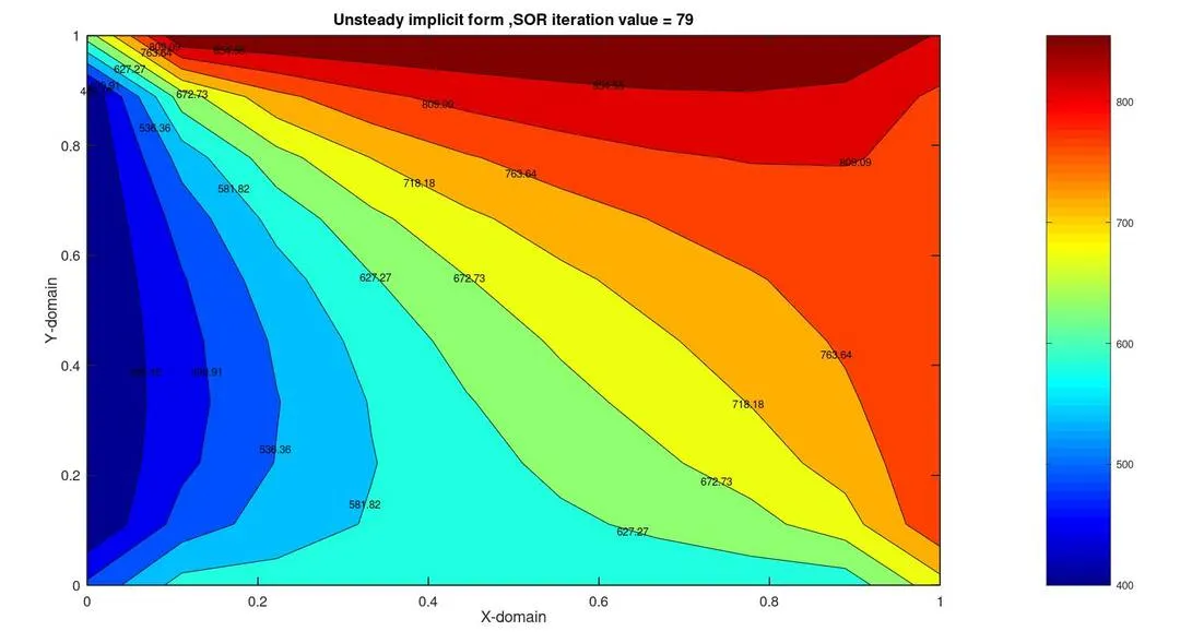
1. It has been found that the Successive over-relaxation method converged faster than the other two methods. It is also to be noted that the relaxation factor in SOR method plays a vital role because applying under relaxation factor takes more iteration than Jacobi and overrelaxation factor makes the solution unstable, so an optimum value of 1.5 was considered to obtain the solution.
2. In unsteady state analysis, both explicit and implicit form showed up the results. But Explicit form cannot be used at all situations. Inorder to obtain the stable solution in explicit form, the total CFL number (k1+k2) should be less than 0.5.
3. From the results, we can clearly say that unsteady state analysis takes more iterations than steady state analysis.