Week 3 - Taylor table method and Matlab code

Coding:

1. The analytical solution of the given function exp(x)*cos(x) has to be compared with the numerical solution of different schemes

2. The value of the derivative is computed at x=pi/3 and forty dx values has been taken between pi/50000 to pi/50.

3. The second derivative of the the given function is found using manual calculations.

4. For a symmetric stencil, the no of nodes = order of approxiation + order of the derivative + 1. So for central differencing the no. of nodes = 5.

5. For an asymmetric stencil, the no. of nodes = order of approxiation + order of the derivative . So for forward and backward differencing the no. of nodes = 6.

6. The Taylor table has been constructed for all the schemes and different equations are obtained for each schemes.

7. The set of linear equations were solved in the Octave using matrix inverse method and passed to the numerical derivative formula.

8. Absolute error is calculated between the anlytical and numerical solution.

9. Different functions are created for each scheme and they are called to the main function and a log graph is plotted between range of dx values and different scheme error values.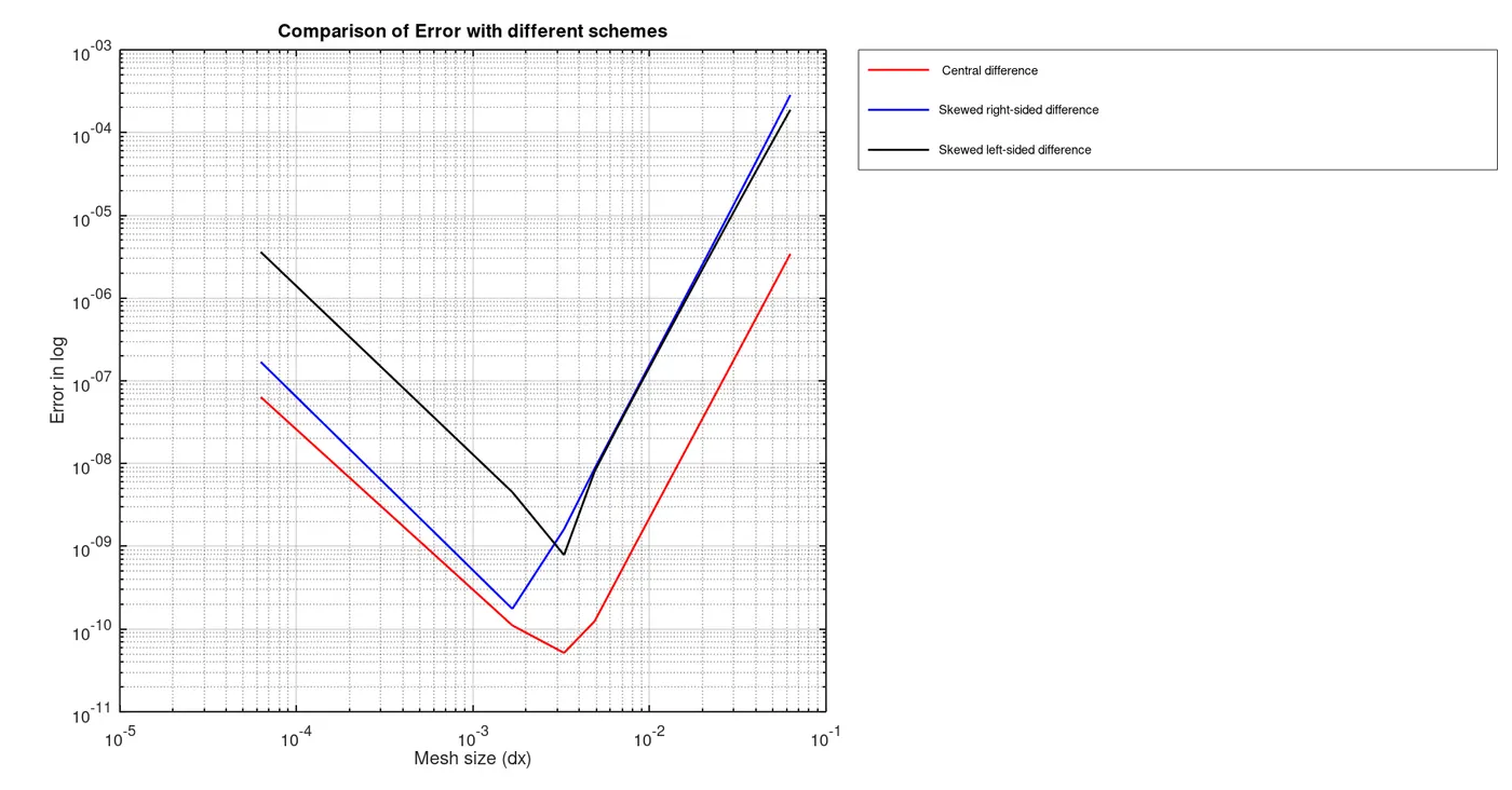

File-1 (Main function)




function backward_differencing_error=backward_differencing_scheme(x,dx)
 
## Finding Analytical solution
  Analytical_solution= -2*exp(x)*sin(x);
  
## Solving for coefficients using Inverse Matrix Method
  y1=[1 1 1 1 1 1;-5 -4 -3 -2 -1 0;25/2 8 9/2 4/2 1/2 0;-125/6 -64/6 -27/6 -8/6 -1/6 0;625/24 256/24 81/24 16/24 1/24 0;-3125/120 -1024/120 -243/120 -32/120 -1/120 0];
  y2=[0 0 1 0 0 0]'
  y3=inv(y1)*y2
  
## Numerical Solution
  a=y3(6)*(exp(x)*cos(x));
  b=y3(5)*(exp(x-dx)*cos(x-dx));
  c=y3(4)*(exp(x-(2*dx))*cos(x-(2*dx)));
  d=y3(3)*(exp(x-(3*dx))*cos(x-(3*dx)));
  e=y3(2)*(exp(x-(4*dx))*cos(x-(4*dx)));
  f=y3(1)*(exp(x-(5*dx))*cos(x-(5*dx))); 
  
  backward_differencing_value = (a+b+c+d+e+f)/(dx^2);
  
## Computing Error
  backward_differencing_error = abs(backward_differencing_value-Analytical_solution)

end









File-2  (Central difference)






function central_differencing_error=central_differencing_scheme(x,dx)
  
## Finding Analytical solution
  Analytical_solution= -2*exp(x)*sin(x);
  
## Solving for coefficients using Inverse Matrix Method
  y1=[1 1 1 1 1;-2 -1 0 1 2 ;2 1/2 0 1/2 2; -4/3 -1/6 0 1/6 4/3; 2/3 1/24 0 1/24 2/3]
  y2=[0 0 1 0 0]'
  y3=inv(y1)*y2
  
## Numerical Solution
  a=y3(1)*(exp(x-(2*dx))*cos(x-(2*dx)));
  b=y3(2)*(exp(x-dx)*cos(x-dx));
  c=y3(3)*(exp(x)*cos(x));
  d=y3(4)*(exp(x+dx)*cos(x+dx));
  e=y3(5)*(exp(x+(2*dx))*cos(x+(2*dx)));

  central_differencing_value = (a+b+c+d+e)/(dx^2);
  
## Computing Error
  central_differencing_error = abs(central_differencing_value-Analytical_solution)
end






File-3 (Forward difference)






function forward_differencing_error=forward_differencing_scheme(x,dx)
  
## Finding Analytical solution
  Analytical_solution= -2*exp(x)*sin(x);
  

## Solving for coefficients using Inverse Matrix Method 
  y1=[1 1 1 1 1 1;0 1 2 3 4 5;0 1/2 2 9/2 8 25/2;0 1/6 8/6 27/6 64/6 125/6;0 1/24 16/24 81/24 256/24 625/24;0 1/120 32/120 243/120 1024/120 3125/120]
  y2=[0 0 1 0 0 0]'
  y3=inv(y1)*y2
  
## Numerical Solution
  a=y3(1)*(exp(x)*cos(x));
  b=y3(2)*(exp(x+dx)*cos(x+dx));
  c=y3(3)*(exp(x+(2*dx))*cos(x+(2*dx)));
  d=y3(4)*(exp(x+(3*dx))*cos(x+(3*dx)));
  e=y3(5)*(exp(x+(4*dx))*cos(x+(4*dx)));
  f=y3(6)*(exp(x+(5*dx))*cos(x+(5*dx)));

  forward_differencing_value = (a+b+c+d+e+f)/(dx^2);

## Computing Error
  forward_differencing_error = abs(forward_differencing_value-Analytical_solution)

  
end







File-4 (Backward difference)



function backward_differencing_error=backward_differencing_scheme(x,dx)
 
## Finding Analytical solution
  Analytical_solution= -2*exp(x)*sin(x);
  
## Solving for coefficients using Inverse Matrix Method
  y1=[1 1 1 1 1 1;-5 -4 -3 -2 -1 0;25/2 8 9/2 4/2 1/2 0;-125/6 -64/6 -27/6 -8/6 -1/6 0;625/24 256/24 81/24 16/24 1/24 0;-3125/120 -1024/120 -243/120 -32/120 -1/120 0];
  y2=[0 0 1 0 0 0]'
  y3=inv(y1)*y2
  
## Numerical Solution
  a=y3(6)*(exp(x)*cos(x));
  b=y3(5)*(exp(x-dx)*cos(x-dx));
  c=y3(4)*(exp(x-(2*dx))*cos(x-(2*dx)));
  d=y3(3)*(exp(x-(3*dx))*cos(x-(3*dx)));
  e=y3(2)*(exp(x-(4*dx))*cos(x-(4*dx)));
  f=y3(1)*(exp(x-(5*dx))*cos(x-(5*dx))); 
  
  backward_differencing_value = (a+b+c+d+e+f)/(dx^2);
  
## Computing Error
  backward_differencing_error = abs(backward_differencing_value-Analytical_solution)

end

Inference:

1. From the graph it has been observed that the error value is always less in central difference scheme than other two schemes because the value at a point is computed using the neighbour values in both directions. Initially the error of skewed right-sided difference is more than skewed left-sided difference but as the dx value changes, the trend of left and right sided difference changes and at the end skewed left sided difference error is more than skewed right sided difference error.

2. But it is not possible to have central difference scheme at all instances because the model is not always symmetric(symmetric stencil is not possible ) , so skewed difference method is applicable in those areas.

3. Symmetric difference method cannot evaluate the value at extreme positions (eg. boundary), so Skewed schemes are better at those positions, because of these constraints it is better to use central differencing at other positions (eg. midway of the model).