Week 7 - Simulation of a 1D Super-sonic nozzle flow simulation using Macormack Method

Simulation of a 1D Super-sonic nozzle flow simulation using Macormack Method

Problem statement: To solve the supersonic nozzle problem through Macormack method in MATLAB or Octave.

Expected results:

1. Perform a grid independence test on the solution and explain all the findings
2. To plot the below mentioned graphs in the report:

• Steady-state distribution of primitive variables inside the nozzle
• Time-wise variation of the primitive variables
• Variation of Mass flow rate distribution inside the nozzle at different time steps during the time-marching process
• Comparison of Normalized mass flow rate distributions of both forms

Background:

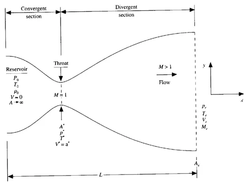
The given nozzle is convergent-divergent type whose length is 3m. Assumption is made in such a way that flow properties would change only in one direction, i.e., along the length of nozzle (X-axis). This is defined as quasi-one-dimensional flow.

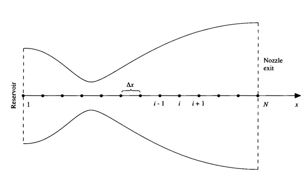
In general, no. of mesh points along the length of the nozzle = 31. Below image shows the grid point distribution along the nozzle.

Maccormack Method:

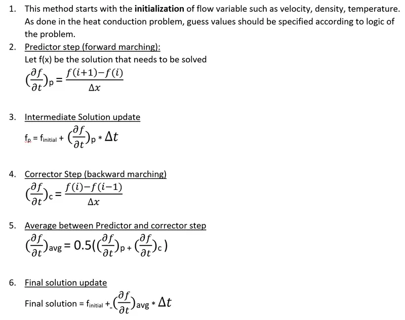
This is a method which provides time marching solution. Below shown is procedure followed to solve the problem until convergence is obtained

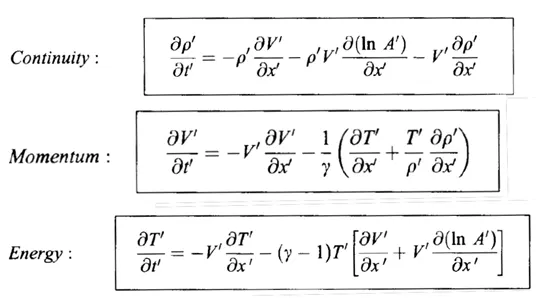
Governing Equations (Non-dimensional form):

• Conservative form

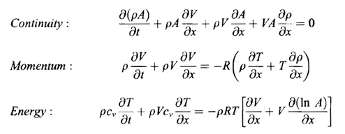
• Non-Conservative form

%Main Function

clear all
close all
clc

%Declaring inputs
n = 31;
x = linspace(0,3,n);
dx = x(2) - x(1);
cfl = 0.5;
nt = 1400;
gamma = 1.4;

%Function call

%Non-Conservative form 
tic
[rho_nc,v_nc,temp_nc,diff_mass_flow_nc,mach_nc,mass_flow_nc,iter_count_nc] = Non_conservative_form(n,x,dx,cfl,nt,gamma);
time_nc=toc

%Conservative form
tic
[rho_c,v_c,temp_c,diff_mass_flow_c,mach_c,mass_flow_c,iter_count_c] = Conservative_form(n,x,dx,cfl,nt,gamma);
time_c=toc

%Plotting Graphs
%Change in Mass flow rate

figure(1)
plot(diff_mass_flow_nc,"linewidth",1);
hold on
plot(diff_mass_flow_c,"linewidth",1);
grid on
xlabel('No.of timesteps');
ylabel('diff Mass flow rate');
set(gca,"linewidth",1,"fontsize",35);
title('Change in Mass flow rate');
legend('Non-conservative form','Conservative form');
set(legend,"location", "northeastoutside","fontsize",35);

%Primitive variables

%Mach No
figure(2)
subplot(2,2,1)
plot(x,mach_nc,"linewidth",2);
hold on
plot(x,mach_c,"linewidth",2,"--");
grid on
xlabel('Distance from Nozzle Inlet (X/L)');
ylabel('Mach no.');
set(gca,"linewidth",1,"fontsize",35);
title('Mach number variation between Conservative & Non-Conservative form');
legend('Non-conservative form','Conservative form');
set(legend,"location", "northeastoutside","fontsize",35);

%Velocity
subplot(2,2,2)
plot(x,v_nc,"linewidth",2);
hold on
plot(x,v_c,"linewidth",2,"--");
grid on
xlabel('Distance from Nozzle Inlet (X/L)');
ylabel('Non-dimensional Velocity');
set(gca,"linewidth",1,"fontsize",35);
title('Velocity variation between Conservative & Non-Conservative form');
legend('Non-conservative form','Conservative form');
set(legend,"location", "northeastoutside","fontsize",35);

%Temperature
subplot(2,2,3)
plot(x,temp_nc,"linewidth",2);
hold on
plot(x,temp_c,"linewidth",2,"--");
grid on
xlabel('Distance from Nozzle Inlet (X/L)');
ylabel('Non-dimensional Temperature');
set(gca,"linewidth",1,"fontsize",35);
title('Temperature variation between Conservative & Non-Conservative form');
legend('Non-conservative form','Conservative form');
set(legend,"location", "northeastoutside","fontsize",35);

%Density
subplot(2,2,4)
plot(x,rho_nc,"linewidth",2);
hold on
plot(x,rho_c,"linewidth",2,"--");
grid on
xlabel('Distance from Nozzle Inlet (X/L)');
ylabel('Non-dimensional Density');
set(gca,"linewidth",1,"fontsize",35);
title('Density variation between Conservative & Non-Conservative form');
legend('Non-conservative form','Conservative form');
set(legend,"location", "northeastoutside","fontsize",35);

%Variation of Mass flow rate between Conservative and Non-Conservative form
figure(3)
plot(x,mass_flow_nc,"linewidth",1);
hold on 
plot(x,mass_flow_c,"linewidth",1);
grid on
xlabel('Distance from Nozzle Inlet (X/L)');
ylabel('Mass flow rate');
set(gca,"linewidth",1,"fontsize",35);
title('Mass flow rate at different grid points');
legend('Non-conservative form','Conservative form');
set(legend,"location", "northeastoutside","fontsize",35);

No_of_iterations_Conservative_form=iter_count_c
No_of_iterations_Non_Conservative_form=iter_count_nc

%Values at throat
disp("Values at throat")
Non_dimensional_Velocity_nc=v_nc(0.5*(n+1))
Non_dimensional_Velocity_c=v_c(0.5*(n+1))
Non_dimensional_density_nc=rho_nc(0.5*(n+1))
Non_dimensional_density_c=rho_c(0.5*(n+1))
Non_dimensional_temperature_nc=temp_nc(0.5*(n+1))
Non_dimensional_temperature_c=temp_c(0.5*(n+1))
Non_dimensional_Mach_no_nc=mach_nc(0.5*(n+1))
Non_dimensional_Mach_no_nc=mach_c(0.5*(n+1))

%Values at Exit
disp("/n Values at Exit")
Non_dimensional_Velocity_nc=v_nc(n)
Non_dimensional_Velocity_c=v_c(n)
Non_dimensional_density_nc=rho_nc(n)
Non_dimensional_density_c=rho_c(n)
Non_dimensional_temperature_nc=temp_nc(n)
Non_dimensional_temperature_c=temp_c(n)
Non_dimensional_Mach_no_c=mach_c(n)
Non_dimensional_Mach_no_nc=mach_nc(n)

% Function for Non-Conservative form

function [rho_nc,v_nc,temp_nc,diff_mass_flow_nc,mach_nc,mass_flow_nc,iter_count_nc] = Non_conservative_form(n,x,dx,cfl,nt,gamma)

%Initial profiles

%Density
rho_nc = 1-0.3146*(x); 

%Temperature              
temp_nc = 1-0.2314*(x);      

%Velocity           
v_nc = (0.1 + 1.09*(x)).*temp_nc.^0.5;

%Area         
a_nc = 1 + 2.2*((x)-1.5).^2;          


%Pre allocation of null matrices
drho_dt_p = zeros(n);
dv_dt_p = zeros(n);
dT_dt_p = zeros(n);

drho_dt_c = zeros(n);
dv_dt_c = zeros(n);
dT_dt_c = zeros(n);

diff_mass_flow_nc = zeros(1,nt);

%Error variables
error_rho = 1e9;
error_v = 1e9;
error_T = 1e9;

%Error tolerance for convergence 
error_tolerance = 1e-5;

iter_count_nc=0;

%Time loop
for k = 1:nt
    
%timestep calculation
dt = min(cfl.*(dx./((temp_nc.^0.5 + v_nc))));

    %Storing initial values
    rho_old = rho_nc;
    T_old = temp_nc;
    v_old = v_nc;
    
  if (error_v > error_tolerance && error_rho > error_tolerance && error_T > error_tolerance)
     
    %Predictor step
    for  j = 2:n-1
        dv_dx = (v_nc(j+1) - v_nc(j))/dx;
        dloga_dx = (log(a_nc(j+1)) -log(a_nc(j)))/dx;
        drho_dx = (rho_nc(j+1) - rho_nc(j))/dx;
        dT_dx = (temp_nc(j+1) - temp_nc(j))/dx;
   
        %Continuity eqn
        drho_dt_p(j) = -rho_nc(j)*dv_dx - rho_nc(j)*v_nc(j)*dloga_dx - v_nc(j)*drho_dx;
       
        %Momentum eqn
        dv_dt_p(j) = -v_nc(j)*dv_dx - (1/gamma)*(dT_dx + (temp_nc(j)/rho_nc(j))*drho_dx);
    
        %Energy eqn
        dT_dt_p(j) = -v_nc(j)*dT_dx - (gamma -1)*temp_nc(j)*(dv_dx + v_nc(j)*dloga_dx);
        
    %Solution update
    rho_nc(j) = rho_old(j) + drho_dt_p(j)*dt;
    v_nc(j) = v_old(j) + dv_dt_p(j)*dt;
    temp_nc(j) = T_old(j) + dT_dt_p(j)*dt;
    endfor
    
    %Corrector step
    for  z = 2:n-1
        dv_dx = (v_nc(z) - v_nc(z-1))/dx;
        dloga_dx = (log(a_nc(z)) -log(a_nc(z-1)))/dx;
        drho_dx = (rho_nc(z) - rho_nc(z-1))/dx;
        dT_dx = (temp_nc(z) - temp_nc(z-1))/dx;
   
        %Continuity eqn
        drho_dt_c(z) = -rho_nc(z)*dv_dx - rho_nc(z)*v_nc(z)*dloga_dx - v_nc(z)*drho_dx;
       
        %Momentum eqn
        dv_dt_c(z) = -v_nc(z)*dv_dx - (1/gamma)*(dT_dx + (temp_nc(z)/rho_nc(z))*drho_dx);
    
        %Energy eqn
        dT_dt_c(z) = -v_nc(z)*dT_dx - (gamma -1)*temp_nc(z)*(dv_dx + v_nc(z)*dloga_dx);
    endfor
    
    %Average values
    drho_dt = 0.5*(drho_dt_p + drho_dt_c);
    dv_dt = 0.5*(dv_dt_p + dv_dt_c);
    dT_dt = 0.5*(dT_dt_p + dT_dt_c);
    
    %Final solution update
    for i = 2:n-1
        rho_nc(i) = rho_old(i) + drho_dt(i)*dt;
        v_nc(i) = v_old(i) + dv_dt(i)*dt;
        temp_nc(i) = T_old(i) + dT_dt(i)*dt;
    endfor
    
    %Boundary conditions
    %Inlet
    v_nc(1) = 2*v_nc(2) - v_nc(3);
    
    %Outlet
    rho_nc(n) = 2*rho_nc(n-1) - rho_nc(n-2);
    v_nc(n) = 2*v_nc(n-1) - v_nc(n-2);
    temp_nc(n) = 2*temp_nc(n-1) - temp_nc(n-2);
    
    %Mach number Evaluation
    mach_nc = v_nc./sqrt(temp_nc); 
    
    %Change in mass flow rate
    diff_mass_flow_nc(k) = rho_nc(1)*a_nc(1)*v_nc(1) - rho_nc(n)*a_nc(n)*v_nc(n);
    
    %Residuals Check
    error_rho = max(abs(rho_nc - rho_old));
    error_v = max(abs(v_nc - v_old));
    error_T = max(abs(temp_nc - T_old));
    
    %No. of iterations update
    iter_count_nc = iter_count_nc+1;

  end
  
    
end
 
%Mass flow rate at different lengths
    mass_flow_nc = rho_nc.*v_nc.*a_nc;
    
endfunction

& Function for Conservative form

function [rho_c,v_c,temp_c,diff_mass_flow_c,mach_c,mass_flow_c,iter_count_c] = Conservative_form(n,x,dx,cfl,nt,gamma)

%Initial profiles
 for i = 1:n
    if (x(i)>=0) && (x(i)<=0.5)
        rho_c(i) = 1;
        temp_c(i) = 1;
    elseif (x(i)>=0.5) && (x(i)<=1.5)
        rho_c(i) = 1 - 0.366*(x(i)-0.5);
        temp_c(i) = 1 - 0.167*(x(i)-0.5);
    elseif (x(i)>=1.5) && (x(i)<=3.2)
        rho_c(i) = 0.634 - 0.3879*(x(i)-1.5);
        temp_c(i) = 0.833 - 0.3507*(x(i)-1.5);
    end
 end

%Area
a_c = 1 + 2.2.*((x-1.5).^2);

%Velocity   
v_c = 0.59./(rho_c.*a_c);              
    

%timestep calculation
x = min(cfl.*(dx./((temp_c.^0.5 + v_c))));
dt=min(x);
 
u1 = rho_c.*a_c;
u2 = rho_c.*a_c.*v_c;
u3 = rho_c.*(temp_c/(gamma-1) + (gamma/2)*(v_c.^2)).*a_c;

%Pre allocation of null matrices
du1_dt_p = zeros(1,n);
du2_dt_p = zeros(1,n);
du3_dt_p = zeros(1,n);
 
j1 = zeros(1,n);
j2 = zeros(1,n);
 
du1_dt_c = zeros(1,n);
du2_dt_c = zeros(1,n);
du3_dt_c = zeros(1,n);
 
diff_mass_flow_c = zeros(1,nt);
iter_count_c = 0;
 
%Error terms
error_v = 1e9;
error_rho = 1e9;
error_temp = 1e9;

%tolerance for convergence
error_tolerance = 1e-5;
  
%Time loop
for k = 1:nt  
    %Storing the initial values
    u1_old = u1;
    u2_old = u2;
    u3_old = u3;
    rho_c_old = rho_c;
    v_c_old = v_c;
    temp_c_old = temp_c;
    f1 = u2;
    f2 = ((u2.^2)./u1) + ((gamma-1)/gamma)*(u3 - ((gamma/2)*(u2.^2)./u1));
    f3 = gamma.*((u2.*u3)./u1) - ((gamma*(gamma-1)/2).*((u2.^3)./u1.^2));
    
if (error_v > error_tolerance && error_rho > error_tolerance && error_temp > error_tolerance)
    
    for i =2:n-1
        j1(i) = (1/gamma)*rho_c(i)*temp_c(i)*(a_c(i+1)-a_c(i))/dx;
    endfor
        
    %Predictor loop
    for j = 2:n-1
        %Continuity equation
        du1_dt_p(j) = -(f1(j+1) - f1(j))/dx;
        
        %Momentum equation
        du2_dt_p(j) = -(f2(j+1) - f2(j))/dx + j1(j);
        
        %Energy equation
        du3_dt_p(j) = -(f3(j+1) - f3(j))/dx;
        
        %Solution update
        u1(j) = u1_old(j) + du1_dt_p(j)*dt;
        u2(j) = u2_old(j) + du2_dt_p(j)*dt;
        u3(j) = u3_old(j) + du3_dt_p(j)*dt;
    endfor
    
    f1 = u2;
    f2 = ((u2.^2)./u1) + ((gamma-1)/gamma)*(u3 - ((gamma/2)*(u2.^2)./u1));
    f3 =  gamma.*((u2.*u3)./u1) - ((gamma*(gamma-1)/2).*((u2.^3)./u1.^2));
     
    for i = 2:n-1
         j2(i) = (1/gamma).*rho_c(i)*temp_c(i)*(a_c(i)-a_c(i-1))/dx;
    endfor
    
    for j = 2:n-1
        %Continuity equation
        du1_dt_c(j) = -(f1(j) - f1(j-1))/dx;
        
        %Momentum equation
        du2_dt_c(j) = -(f2(j) - f2(j-1))/dx + j2(j);
        
        %Energy equation
        du3_dt_c(j) = -(f3(j) - f3(j-1))/dx;
    endfor
    
    %Calculating the average values
    du1_dt_avg = 0.5*(du1_dt_p + du1_dt_c);
    du2_dt_avg = 0.5*(du2_dt_p + du2_dt_c);
    du3_dt_avg = 0.5*(du3_dt_p + du3_dt_c);
    
    for i = 2:n-1
        u1(i) = u1_old(i) + du1_dt_avg(i)*dt;
        u2(i) = u2_old(i) + du2_dt_avg(i)*dt;
        u3(i) = u3_old(i) + du3_dt_avg(i)*dt;
    end
    
    %Applying boundary conditions
    %Inlet
    u2(1) = 2*u2(2) - u2(3);
    
    %Outlet
    u1(n) = 2*u1(n-1) - u1(n-2);
    u2(n) = 2*u2(n-1) - u2(n-2);
    u3(n) = 2*u3(n-1) - u3(n-2);
    
    %Primitive variables Evaluation
    
    %Density
    rho_c = u1./a_c;
    
    %Velocity
    v_c = u2./(rho_c.*a_c);
    
    %Temperature
    temp_c = (gamma-1)*((u3./u1) - (gamma/2)*v_c.^2);
    
    %Mach number
    mach_c = v_c./sqrt(temp_c);
    
    %Net mass flow rate
    diff_mass_flow_c(k) = rho_c(1)*v_c(1)*a_c(1) - rho_c(n)*v_c(n)*a_c(n);
    
    %Residuals Check
    error_rho = max(abs(rho_c - rho_c_old));
    error_v = max(abs(v_c - v_c_old));
    error_temp = max(abs(temp_c - temp_c_old));
    
    %No. of iterations update
    iter_count_c = iter_count_c+1;
  end 
    
end
%Mass flow along the length of Nozzle
    mass_flow_c = rho_c.*v_c.*a_c;
    
    
endfunction

Results & Discussions:

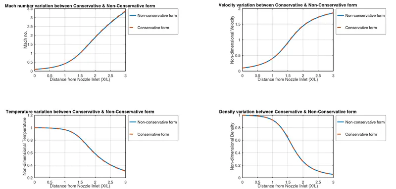
From the above graphs, flow variable such as Mach Number, Velocity, temperature, and Density values does not vary between Conservative and Non-Conservative form.

Since it is a Convergent divergent nozzle, the flow at the inlet would be subsonic, at the throat it would be sonic and at the outlet it would be supersonic. It is well proven from the Mach No graph. Since Mach no is a function of Velocity of the fluid, the trend of velocity curve would also be same as Mach No.

The temperature value would be higher at the inlet (Reservoir end). Since pressure value is lesser at the outlet of the nozzle (Pressure is inversely proportional to velocity), the temperature is also lesser at the outlet. Density curve trend is similar to the temperature curve.

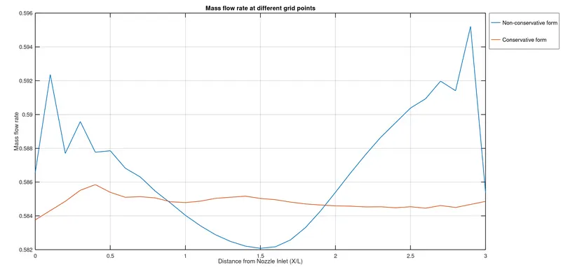
Above graph shows the mass flow rate change between Conservative and Non-Conservative form. The mass flow rate ranges between 0.58 to 0.59 which is almost consistent. But in Non-conservative form the fluctuations are higher at the inlet and outlet of the nozzle.

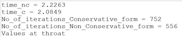
Time taken for Non-conservative program to get executed: 2.2263 seconds

Time taken for Conservative program to get executed: 2.0849 seconds

Though the no. of iterations seems to higher for Conservative form, computational time is less. So, from above explanations, we can conclude that Conservative form is much stable than Non-Conservative form.

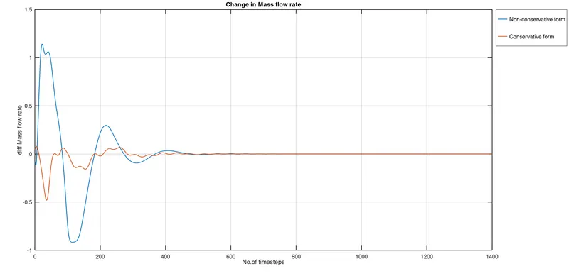
The above graph shows the change in mass flow out – mass flow in between conservative and non-conservative form for different time steps. Initially the variation is higher for Non-conservative form. In both the forms after 400^th timestep, the value becomes stabilized.

Grid Independence study:

The graphs and results discussed above is for 31 grid points.

Below table shows the difference in primitive variables obtained between conservative and non-conservative form for different grid points

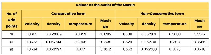
As the no. of grid points increases, the solution is becoming more accurate. But the computational time is also increasing.

Results from Grid Independence test:

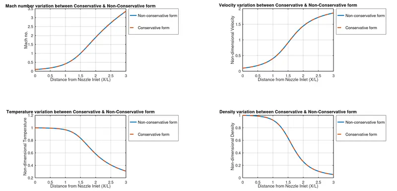
• No. of Grid Points: 61

• No. of Grid Points: 91

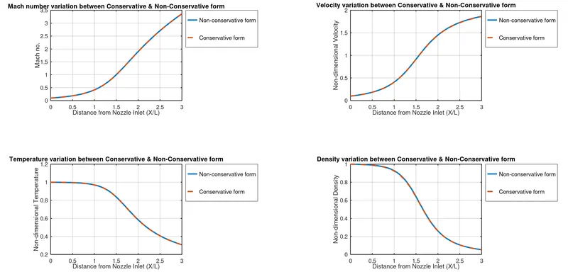
There is no much change in trend between different grid points graphs.So increasing the no of grid points is not significant with the results obtained for this case.

Conclusion:

From the results obtained, it can be concluded that Conservative form is more accurate than the Non-Conservative form in terms of solution obtained. Also the Convergent-Divergent nozzle supersonic flow is properly obtained through the Macormack Method.