Week 9 - FVM Literature Review
Objective: A literature review on Finite Volume Method and also explain the interploitaion schemes and flux limiters.
`text(Finite Volume Method)`
`text(Finite volume method provide a efficient way of discretizing the governing equations to solve certain Heat Transfer and Fluid flow problems. FVM is similar to Finite Difference Method(FDM) technique wherein derivative are written in form of the differences that is applied on the points/nodes. FVM applies the same concept but here in FVM derivatives which are discretized are applied to the volumes. FVM compute solution at each finite volume where FDM computes solution at each points/nodes. Here in FVM governing equations solved in an integral form so it serves to conserve the properties in a better way than FDM. FVM is based on the laws of conservation and hence one end up with a formulation consisting of flux conservation equations. FVM is the computation method of evaluating the represented system of PDEs at discrete places on a meshed geometry . As the names suggests, small or finite-sized volume surrounding each point on a mesh is formulated. The strength of FVM is that it only needs to evaluate the flux for the cell boundaries and is applicable to non-linear problems which makes it a preferred choice due to its computational power and robustness in handling both linear and non-linear conservation laws appearing in the transport equation. The local accuracy of the FVM can be improved by refining the mesh at the region of interest which cannot be performed in the FDM. However the FVM can not easily compute an approximation o the solution when the order is increase whereas other Finite Element Method and Finite Difference Method performs efficiently in such cases. In FVM, volume integral are converted to surface integrals using divergence theorem , which is then evaluated as fluxes at the surface of each finite volume. As it follow the laws of conservation , the flux entering a volume is identical to the flux leaving the volume.)`
`text(Interpolation Schemes:)`
`text(The approximation of surface and volume integrals may require valves of the variable at the location other than the computational nodes of the control volume . Values at variable at the location are obtained by the interpolation scheme. For example. 1D linear Heat conduction equation in steady state, the source and alpha values are function of temperature and we need to calculate the temperatures separately to the that particular face by taking the temperature from the adjoining cells by the usages of interpolation scheme. Now let is look at the different interpolation scheme.)`
`text(1. Upwind difference approximation scheme: It is used for calculation the approximate value of the variable at the east face of the control volume. It is first order accurate and is numerically diffusive with coefficient of numerical diffusion.)`
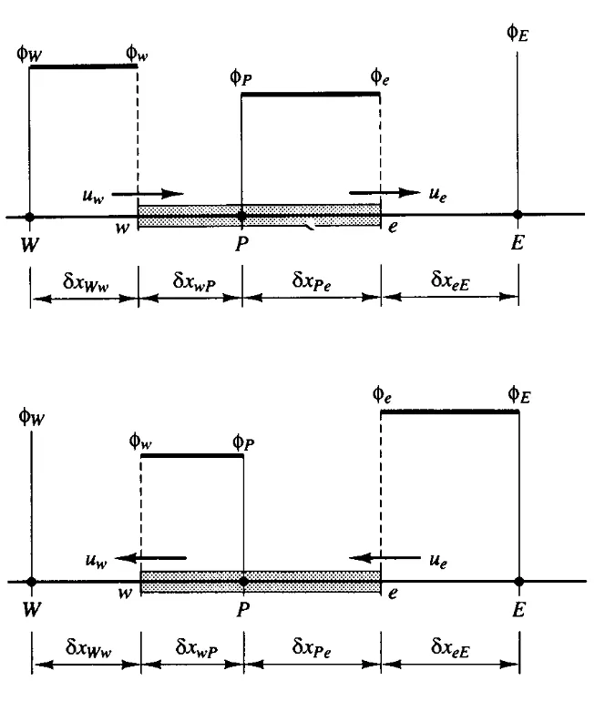
When the flow is positive direction
`u_{w\ }>0,u_e>\ 0 (F_w>\ 0\ ,\ F_e>\ 0)`
the upwind scheme set as
`phi_{w\ }=phi_W` and `phi_{e\ }=phi_P`
1. `(u_i^{n+1}\ -\ u_i^n)/(Deltat)\ +\ a(u_i^n\ -\ u_{i-1)^n)/(Deltax)\ =\ 0\ text(for)\ a>\ 0`
2. `(u_i^{n+1}\ -\ u_i^n)/(Deltat)\ +\ a(u_(i+1)^n\ -\ u_{i)^n)/(Deltax)\ =\ 0\ text(for)\ a<\ 0`
2.Linear upwind difference approximation scheme: When an upwind scheme is second order accurate , it known as LUDS. To improve the spatial accuracy of the upwind difference or first order upwind scheme . 3 data points are considered instead of 2. This reuslts in higher accuracy in approximating the spatial derivatives . This scheme has also been noticed to be less diffusive than the first order upwind scheme .
`u_x^-` = `(3u_i^n -4u_(i-1)^n + u_(i-2)^n)/(2Deltax)`
`u_x^+` = `(-u_(i+2)^n + 4u_(i+1)^n + 3u_(i)^n) / (2Deltax)`
3. Quardratic Upwind difference approximation scheme: Quadratic upwind difference approximation scheme is known as quadratic upwind interpolation for convective kinematics (QUICK). This is a hogher order differncing scheme which considers 3 data points weighted quadratic interpolation for the cell face vaues . it performs a third order flux approximation and has an overall accuracy of second order . it is considered to be marginally better than the LUDS. However , it introduce slight instabilities in the region with high gradient.
`u_x^-` = `(2u_(i+1)^n + 3u_(i)^n - 6u_(i-1)^n + u_(i-2)^n)/ (6Deltax)`
`u_x^+` = `(-u_(i+2)^n + 6u_(i+1)^n - 3u_(i)^n + 2u_(i-1)^n)/ (6Deltax)`
4.Central differencing approximation scheme : this scheme is relatively easier to implement and provides with fasters convergence rate as compared to other schemes . It also has higher accuracy than the first order upwind scheme if the peclet number is less than 2.
Interpolational Polynomial
`p_1(x) = u_l (x_R - x)/(x_R - x_L) + u_R (x - x_L)/(x_R - x_L)`
Averged interface values
`u_(i-1/2)` `~~ (u_(i-1) + u_i)/2 , u_(i+1/2) ~~( u_i + u_(i+1))/2`
`I_c ~~ v(u_(i+1) - u_(i-1))/(2Deltax)`
`text(Flux Limiters:)`
`text(Flux limiters are used mainly to limit the values of flux quantities which can tend to oscillate and give unrealistic values due to shocks , discontinuities and sharp changes in the solution domain . The use of flux limiters makes the solution total variable diminishing. The main idea behind the construction of flux limiters scheme is to limit the spatial derivatives to realistic values. They are used I high-resolution scheme for solving problems described by PDEs and only come into operation when sharp wavefronts are present . Form smoothly changing waves , the flux limiters do not operate and the spatial derivatives can be represented by higher order approximation without introducing spurious oscillations. Commonly used flux limiters are`
a) Minmod
b) Superbee
c) CHARM
d) HQUICK
e) Van Leer)`