Week 7 - Simulation of a 1D Super-sonic nozzle flow simulation using Macormack Method
`text(Objective : To simulate the isentropic flow through a Quassi 1-D super-sonic nozzle by deriving both the conservation and non-conservation forms of governing equation and solve them by implementing the macCormack's technique using MATLAB).`
`text( Subsonic and supersonic isentropic flow through the convergence and divergence nozzle)`
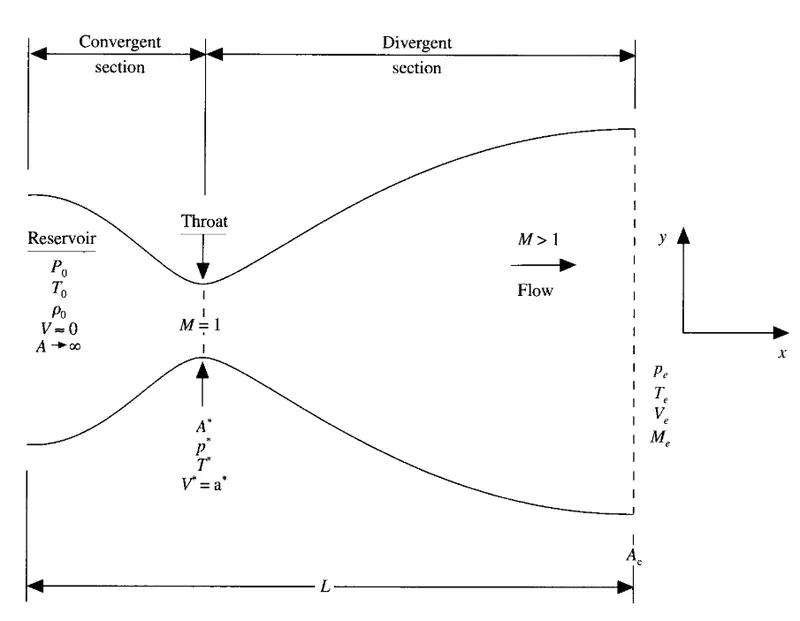
`text( Conservative form)`
`text(Continuity Equation) :` `(del(rhoprimeAprime))/(del tprime)+(del(rhoprimeAprimeVprime))/(delxprime) = 0`
`text(Momentum Equation) :``(del(rhoprimeAprimeVprime))/(deltprime) + (del(rhoprimeAprimeV^2+1/gammapprimeAprime))/(delxprime) = 1/gammapprime(delAprime)/(delxprime)`
`text(Energy Equation) :``(del[rhoprime((Tprime)/(gamma-1)+gamma/2V^2)Aprime])/(deltprime) + (del[rhoprime((Tprime)/(gamma-1)+gamma/2V^2)VprimeAprime+rhoprimeAprimeVprime])/(delxprime) = 0`
`text(Non-Conservation Form)`
`text(Continuity Equation) :` `(delrhoprime)/(deltprime) = rhoprime(delVprime)/(delxprime) - rhoprimeVprime(del(lnA))/(delxprime) - Vprime(delrhoprime)/(delxprime)`
`text(Momentum Equation) :``(delVprime)/(deltprime) = Vprime(delVprime)/(delxprime) - 1/gamma((delTprime)/(delxprime)+(Tprime)/(rhoprime)(delrhoprime)/(delxprime))`
`text(Energy Equation) :``(delTprime)/(deltprime) = Vprime(delTprime)/(delxprime) - (gamma-1)Tprime[(delVprime)/(delxprime) + Vprime(del(lnAprime))/(delxprime)]`
`text(MacCormack's Method)`
`text(MacCormack's method help to descritize the numerical solution of governing equation.It is proceed with two step i.e. Predictor step and Corrector step and solve the governing equation in much simpler way. )`
`text(In predictor step, we use forward difference method is spatial term and in corrector step, we use backward difference method in spatial term and having time step)``Deltat`
Main Code
close all

clc

%input
n = 31;
gamma = 1.4;
x = linspace(0,3,n);
%grid
dx = x(2)-x(1);
a = 1+(2.2*(x-1.5).^2);
nt = 1400;
%courant number
C = 0.5;


%calculation
 tic;
[v_nc,T_nc,rho_nc,mass_flow_rate_nc,mach_nc,p_nc,rho_throat_nc,v_throat_nc,T_throat_nc,mach_throat_nc,p_throat_nc,mass_flow_rate_throat_nc] = non_conservative_form(x, dx, n, gamma, nt, C);
sim_time_nc = toc;
fprintf('sim time for non conservative form: %f',sim_time_nc);
hold on

%plotting

%Time step variation of properties at throat area in nc

figure(2)
hold on
%Density
subplot(5,1,1)
plot(linspace(1,nt,nt),rho_throat_nc,'Color','m');
ylabel('Density');
legend({'Density at throat'});
axis([0  1400  0  1.3]);
grid minor;
title('Time step variation at throat area - non conservative');

%Temperature
subplot(5,1,2)
plot(linspace(1,nt,nt),T_throat_nc,'Color','c');
ylabel('Temperature');
legend({'Temperature at throat'});
axis([0  1400  0.6  1]);
grid minor;

%pressure
subplot(5,1,3)
plot(linspace(1,nt,nt),p_throat_nc,'Color','g');
ylabel('pressure');
legend({'pressure at throat'});
axis([0  1400  0.4  1.1]);
grid minor

%mach number
subplot(5,1,4)
plot(linspace(1,nt,nt),mach_throat_nc,'Color','y');
xlabel('Time step')
ylabel('mach number');
legend({'mach number at throat'});
axis([0  1400  0.6  1.4]);
grid minor;

%Velocity
subplot(5,1,5)
plot(linspace(1,nt,nt),v_throat_nc,'Color','k');
ylabel('velocity');
legend({'velocity at throat'});
axis([0  1400  0  1.5]);
grid minor;

% Steady state simulation for primitive values for non conservation form

figure(3);
hold on
%Density
subplot(5,1,1)
plot(x,rho_nc,'Color','m');
ylabel('Density');
legend({'Density'});
axis([0 3 0 1]);
grid minor;
title(' variation of flow rate distribution - non conservative');

%Temperature
subplot(5,1,2)
plot(x,T_nc,'Color','c');
ylabel('Temperature');
legend({'Temperature'});
axis([0 3 0 1]);
grid minor;

%pressure
subplot(5,1,3)
plot(x,p_nc,'Color','g');
ylabel('pressure');
legend({'pressure '});
axis([0 3 0 1]);
grid minor;

%mach number
subplot(5,1,4)
plot(x,mach_nc,'Color','y');
xlabel('Nozzle length')
ylabel('mach number');
legend({'mach number'});
axis([0 3 0 4]);
grid minor;

%Velocity
subplot(5,1,5)
plot(x,v_nc,'Color','k');
ylabel('velocity');
legend({'velocity '});
 axis([0  3  0  2]);
grid minor;


% Function for conservative form
tic;
[v_c, T_c, rho_c, mass_flow_rate_c, mach_c,p_c, rho_throat_c, v_throat_c, T_throat_c,mach_throat_c,p_throat_c,mass_flow_rate_throat_c] = conservative_form(x,dx,n,gamma,nt,C);
sim_time_c = toc;
fprintf('sim time for conservative form: %f',sim_time_c);
hold on
%Plotting

%Time step variation of properties at throat area in c
figure(5)
hold on
%Density
subplot(5,1,1)
plot(rho_throat_c,'Color','m');
ylabel('Density');
legend({'Density at throat'});
axis([0  1400  0  1.3]);
grid minor;
title('Time step variation at throat area -  conservative form');

%Temperature
subplot(5,1,2)
plot(T_throat_c,'Color','c');
ylabel('Temperature');
legend({'Temperature at throat'});
axis([0  1400  0.6  1]);
grid minor;

%pressure
subplot(5,1,3)
plot(p_throat_c,'Color','g');
ylabel('pressure');
legend({'pressure at throat'});
axis([0  1400  0.2  0.8]);
grid minor;

%mach number
subplot(5,1,4)
plot(mach_throat_c,'Color','y');
xlabel('Time step')
ylabel('mach number');
legend({'mach number at throat'});
axis([0  1400  0.6  1.4]);
grid minor;

%Velocity
subplot(5,1,5)
plot(v_throat_c,'Color','k');
ylabel('velocity');
legend({'velocity at throat'});
 axis([0  1400  0.85  0.95]);
grid minor;

% Steady state simulation for primitive values for conservation form
figure(6)
hold on
%Density
subplot(5,1,1)
plot(x,rho_c,'Color','m');
ylabel('Density');
legend({'Density'});
axis([0 3 0 1]);
grid minor;
title(' variation of flow rate distribution -  conservative form');

%Temperature
subplot(5,1,2)
plot(x,T_c,'Color','c');
ylabel('Temperature');
legend({'Temperature'});
axis([0 3 0 1]);
grid minor;

%pressure
subplot(5,1,3)
plot(x,p_c,'Color','g');
ylabel('pressure');
legend({'pressure '});
axis([0 3 0 1]);
grid minor;

%mach number
subplot(5,1,4)
plot(x,mach_c,'Color','y');
xlabel('Nozzle length')
ylabel('mach number');
legend({'mach number'});
axis([0 3 0 4]);
grid minor;

%Velocity
subplot(5,1,5)
plot(x,v_c,'Color','k');
ylabel('velocity');
legend({'velocity '});
axis([0  3  0  2]);
grid minor;

% comparision plot of normalized mass flow rate of both the form
 figure(7)
  hold on
 plot(x,mass_flow_rate_nc,'r','LineWidth',1.25);

 plot(x,mass_flow_rate_c,'b','LineWidth',1.25);

 legend('Non conservative form','conservative form');
xlabel('length of the domain');
ylabel('mass flow rate');
title('comparision plot of normalized mass flow rate of both the form');
Conservation form
function [v_c,T_c,rho_c,mass_flow_rate_c,mach_c,p_c,rho_throat_c,v_throat_c,T_throat_c,mach_throat_c,p_throat_c,mass_flow_rate_throat_c] = conservative_form(x,dx,n,gamma,nt,C,throat,a)
%input
n = 31;
x = linspace(0,3,n);
%grid
dx = x(2)-x(1);
a = 1+(2.2*(x-1.5).^2);
%courant number
C = 0.5;
gamma = 1.4;
nt = 1400;

%Determining initial profile of density and temperature
for i = 1:n
    if (x(i)>=0 && x(i)<=0.5)
        rho_c(i) = 1;
        T_c(i) = 1;
    elseif (x(i)>=0.5 && x(i)<=1.5)
        rho_c(i) = 1-0.366*(x(i)-0.5);
        T_c(i) = 1-0.167*(x(i)-0.5);
    elseif (x(i)>=1.5 && x(i)<=3)
        rho_c(i) = 0.634-0.3879*(x(i)-1.5);
        T_c(i) = 0.833-0.357*(x(i)-1.5) ;
    end
end

%area and throat profile
a = 1+(2.2*(x-1.5).^2);
throat = round(n/2);
% Initial profile for velocity and pressure
v_c = 0.59./(rho_c.*a);
p_c = rho_c.*T_c;

%calculation the initial solution vectors
U1 = rho_c.*a;
U2 = rho_c.*a.*v_c;
U3 = rho_c.*a.*(T_c./(gamma-1))+((gamma/2).*v_c.^2);

%outer time loop
for k =1:nt
    dt = max(C.*dx./(sqrt(T_c) + v_c));
    %solving a copy of old values
    U1_old = U1;
    U2_old = U2;
    U3_old = U3;
    % calculating the flux vector
    F1 = U2;
    F2 = ((U2.^2)./U1) + ((gamma-1)/gamma)*(U3-(gamma/2)*((U2.^2)./U1));
    F3 = ((gamma*U2.*U3)./U1) - (gamma*(gamma-1)*((U2.^3)./(2*U1.^2)));

    %predictor method
for j = 2:n-1
    %calculating the source term
    J2(j) = (1/gamma)*rho_c(j)*T_c(j)*((a(j+1)-a(j))/dx);
    % continuity equation
    dU1_dt_p(j) = -((F1(j+1)-F1(j))/dx);
    %momentum equation
    dU2_dt_p(j) = -((F2(j+1)-F2(j))/dx) + J2(j);
    %energy equation
    dU3_dt_p(j) = -((F3(j+1)-F3(j))/dx);

    %updating new value
     U1(j) = U1(j) + dU1_dt_p(j)*dt;
     U2(j) = U2(j) + dU2_dt_p(j)*dt;
     U3(j) = U3(j) + dU3_dt_p(j)*dt;


end

  %updating flux vector
    F1 = U2;
    F2 = ((U2.^2)./U1) + ((gamma-1)/gamma)*(U3-(gamma*0.5*(U2.^2))./(U1));
    F3 = ((gamma*U2.*U3)./U1) - ((gamma*0.5*(gamma-1)*(U2.^3))./(U1.^2));

    %corector method
for j = 2:n-1
    %calculating the source term
    J2(j) = (1/gamma)*rho_c(j)*T_c(j)*((a(j)-a(j-1))/dx);
    % continuity equation
    dU1_dt_c(j) = -((F1(j)-F1(j-1))/dx);
    %momentum equation
    dU2_dt_c(j) = -((F2(j)-F2(j-1))/dx) + J2(j);
    %energy equation
    dU3_dt_c(j) = -((F3(j)-F3(j-1))/dx);
end
    %compute average time derivative
   dU1_dt = 0.5*(dU1_dt_p + dU1_dt_c);
   dU2_dt =0.5*(dU2_dt_p + dU2_dt_c);
   dU3_dt =0.5*(dU3_dt_p + dU3_dt_c);

   %Final solution update
for i = 2:n-1
   U1(i) = U1_old(i) + dU1_dt(i)*dt;
    U2(i) = U2_old(i) + dU2_dt(i)*dt;
    U3(i) = U3_old(i) + dU3_dt(i)*dt;
end


    %Applying boundary condition\
    % at inlet
    U1(1) = rho_c(1)*a(1);
    U2(1) = 2*U2(2) - U2(3);
    v_c(1) = U2(1)./U1(1);
    U3(1) = U1(1)*((T_c(1)/(gamma-1)) + ((gamma/2)*(v_c(1)).^2));
    %at outlet
    U1(n) = 2*U1(n-1) - U1(n-2);
    U2(n) = 2*U2(n-1) - U2(n-2);
    U3(n) = 2*U3(n-1) - U3(n-2);

    %Final primitive variable
    rho_c = U1./a;
    v_c = U2./U1;
    T_c = (gamma-1)*((U3./U1 - (gamma/2)*(v_c).^2));
    %define mass flow rate ,pressure and mach number
    mass_flow_rate_c = rho_c.*a.*v_c;
    p_c = rho_c.*T_c;
    mach_c = (v_c./sqrt(T_c));
    %calculating variable at throat section
    rho_throat_c(k) = rho_c(throat);
    v_throat_c(k) = v_c(throat);
    T_throat_c(k) = T_c(throat);
    mass_flow_rate_throat_c(k) = mass_flow_rate_c(throat);
    p_throat_c(k) = p_c(throat);
    mach_throat_c(k) = mach_c(throat);

    figure(4)
hold on
if k == 50
    plot(x, mass_flow_rate_c,'m','LineWidth',1.25);

elseif k== 100
      plot(x, mass_flow_rate_c,'c','LineWidth',1.25);

elseif k== 200
      plot(x, mass_flow_rate_c,'g','LineWidth',1.25);

elseif k== 500
      plot(x, mass_flow_rate_c,'y','LineWidth',1.25);

elseif k== 800
      plot(x, mass_flow_rate_c,'k','LineWidth',1.25);

end

%labelling
title('mass flow rate at different time step conservative form');
xlabel('Distance');
ylabel('mass flow rate');
legend('time step = 50','time step = 100','time step = 200','time step = 500','time step = 800');
axis([0 3 0.4 1])

end
end
Non-Conservation form
%Function for non conservative form
function[v_nc,T_nc,rho_nc,mass_flow_rate_nc,mach_nc,p_nc,rho_throat_nc,v_throat_nc,T_throat_nc,mach_throat_nc,p_throat_nc,mass_flow_rate_throat_nc]= non_conservative_form(x,dx,n,gamma,nt,C)
 %input
n = 31;
x = linspace(0,3,n);
%grid
dx = x(2)-x(1);
a = 1+(2.2*(x-1.5).^2);
%courant number
C = 0.5;
gamma = 1.4;
nt = 1400;
%Initial  condition
rho_nc = 1-0.3146*x;
T_nc = 1-0.2341*x;
v_nc = (0.1+1.09*x).*T_nc.^0.5;
%area and throat profile
a = 1+2.2*(x-1.5).^2;
throat =find(a==1);
%outer time loop
for k = 1:nt
    %time-step control
    dt = min(C.*dx./(sqrt(T_nc)+v_nc));
    %saving a copy of old values
    rho_old = rho_nc;
    T_old = T_nc;
    v_old = v_nc;

%predictor method
for j = 2:n-1
    %simplifying the equation spatial terms
    dv_dx = (v_nc(j+1)-v_nc(j))/dx;
    drho_dx = (rho_nc(j+1)-rho_nc(j))/dx;
    dT_dx = (T_nc(j+1)-T_nc(j))/dx;
    dlog_a_dx = (log(a(j+1))-log(a(j)))/dx;

    %Continuity equation
    drho_dt_p(j) = -rho_nc(j)*dv_dx-rho_nc(j)*v_nc(j)*dlog_a_dx - v_nc(j)*drho_dx;

    %Mometum equation
    dv_dt_p(j) = -v_nc(j)*dv_dx - (1/gamma)*(dT_dx+(T_nc(j)*drho_dx/rho_nc(j)));

    %Energy equation
    dT_dt_p(j) = -v_nc(j)*dT_dx - (gamma-1)*T_nc(j)*(dv_dx + v_nc(j)*dlog_a_dx);

   %solution update
   rho_nc(j) = rho_nc(j) + drho_dt_p(j)*dt;
v_nc(j) = v_nc(j) + dv_dt_p(j)*dt;
T_nc(j) = T_nc(j) + dT_dt_p(j)*dt;

end
%corrector Method
for j = 2:n-1
    %simplifying the equation spatial terms
    dv_dx = (v_nc(j)-v_nc(j-1))/dx;
    drho_dx = (rho_nc(j)-rho_nc(j-1))/dx;
    dT_dx = (T_nc(j)-T_nc(j-1))/dx;
    dlog_a_dx = (log(a(j))-log(a(j-1)))/dx;

    %Continuity equation
    drho_dt_c(j) = -rho_nc(j)*dv_dx-rho_nc(j)*v_nc(j)*dlog_a_dx - v_nc(j)*drho_dx;

    %Mometum equation
    dv_dt_c(j) = -v_nc(j)*dv_dx - (1/gamma)*(dT_dx+(T_nc(j)*drho_dx/rho_nc(j)));

    %Energy equation
    dT_dt_c(j) = -v_nc(j)*dT_dx - (gamma-1)*T_nc(j)*(dv_dx + v_nc(j)*dlog_a_dx);
end
%compute average time derivative
  drho_dt = 0.5.*(drho_dt_p + drho_dt_c);
   dv_dt =0.5.*(dv_dt_p + dv_dt_c);
   dT_dt =0.5.*(dT_dt_p + dT_dt_c);

   %Final solution update
for i = 2:n-1
   rho_nc(i) = rho_old(i) + drho_dt(i)*dt;
v_nc(i) = v_old(i) + dv_dt(i)*dt;
T_nc(i) = T_old(i) + dT_dt(i)*dt;
end

%Apply boundary condition
%at inlet
rho_nc(1) = 1;
v_nc(1) = 2*v_nc(2) - v_nc(3);
T_nc(1) = 1;
% at outlet
rho_nc(n) = 2*rho_nc(n-1) - rho_nc(n-2);
v_nc(n) = 2*v_nc(n-1) - v_nc(n-2);
T_nc(n) = 2*T_nc(n-1) - T_nc(n-2);
%defin mass flow rate ,pressure and mach number
mass_flow_rate_nc = rho_nc.*a.*v_nc;
p_nc = rho_nc.*T_nc;
mach_nc = (v_nc./sqrt(T_nc));
%calculating variable at throat section
rho_throat_nc(k) = rho_nc(throat);
v_throat_nc(k) = v_nc(throat);
T_throat_nc(k) = T_nc(throat);
mass_flow_rate_throat_nc(k) = mass_flow_rate_nc(throat);
p_throat_nc(k) = p_nc(throat);
mach_throat_nc(k) = mach_nc(throat);
%plotting
%comparision of non-dimensional mass flow rate at different time step
figure(1)
 hold on
if k == 50
    plot(x, mass_flow_rate_nc,'m','LineWidth',1.25);

elseif k== 100
      plot(x, mass_flow_rate_nc,'c','LineWidth',1.25);

elseif k== 200
      plot(x, mass_flow_rate_nc,'g','LineWidth',1.25);

elseif k== 500
      plot(x, mass_flow_rate_nc,'y','LineWidth',1.25);

elseif k== 800
      plot(x, mass_flow_rate_nc,'k','LineWidth',1.25);

end

%labelling
title('mass flow rate at different time step non-conservation form');
xlabel('Distance');
ylabel('mass flow rate');
legend('time step = 50','time step = 100','time step = 200','time step = 500','time step = 800');
axis([0 3 0.2 2])

end
end
Plot
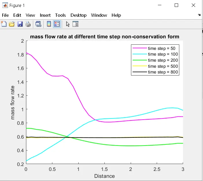
1) Mass flow rate at different time step - non-conservation form
2) Mas flow rate at different time step - Conservation form
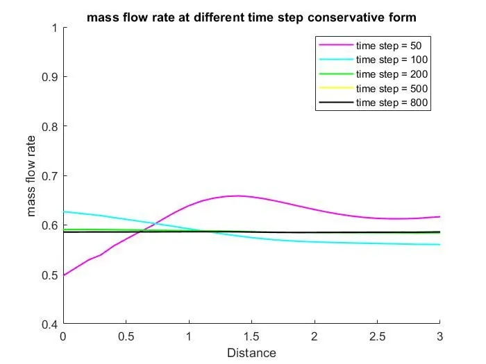
Both plot shows that mass flow rate at different tie step. It seems that after time step 200 solution become stable.
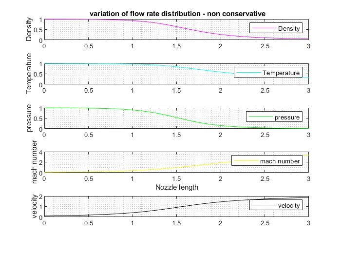
3) Variation of flow rate distribution - non-conservative form
4) Variation of flow rate distribution - conservative form
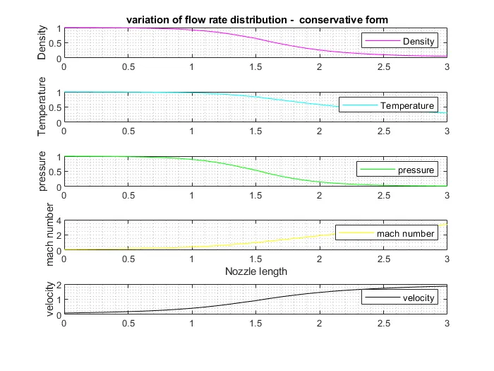
above plots for the both form is same showing exact same solution for all the values.
5) Time step variation at throat area - non-conservative form
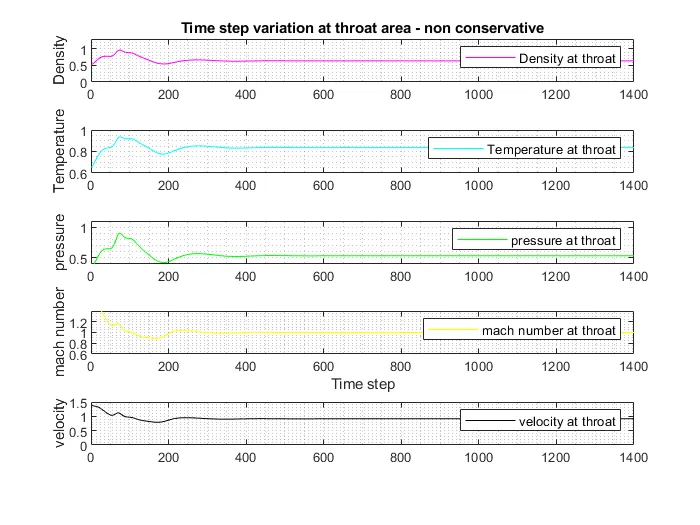
6) Time step variation at throat area -conservative form
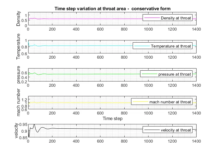
From aove plot we can say that non-conservative form taking more time to achieve solution as compared to the conservative form.
7) Comparision plot of normalized mass flow rate of both the form
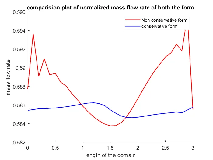
From the above plot we can see that Conservative form attains faster staility than non-conservative form . Non-conservative form takes long length to reach the stable solution and conservative form take less length to reach the stable solution.
Conclusion:
From the all observation we can say that conservatve form converges faster than non-conservative form by giving the stable solution.Simulation time for conservative form is less then non-conservative form.There is no much effect of changing the grid point on the solution.