Week 9 - FVM Literature Review
Aim: To study and explain
(i) What is Finite Voulume Method (FVM)?
(ii) State the major differences between FDM & FVM.
(iii) State the necessity of interpolation schemes in FVM and their types.
(iv) What is flux limiter in FVM & what is its need if FVM.
Theory:
1) Finite Volume Method (FVM):
In this method the computational domain is divided into finite number of non overlapping control volumes and define the computational nodes at which the variables are to be evaluated.
Then apply the integral form of governing equations to the each control volume this gives the discretised equation at the node corresponding to respective control volume.
Approximate the surface and volume integrals using appropriate quadrature formulae in terms of the function values at computational nodes.
The discretised equations are obtained for all computational nodal points to solve the problem. The equations for finite volumes adjacent to the domain boundaries are obtained with the help of boundary conditions. Then this system of algebraic equations is solved using any suitable matrix solution technique. The values of variable ( here `phi`) at each nodal point are obtained.
There are two common approaches to finite volume discretisation i.e.
(a) Cell centered approach: Control volumes are defined by a suitable grid and computational nodes are assigned at the control volume centroids. It can be used with structured or unstructured grids thus more commonly used.
(b) Face Centered approach: Nodal locations are defined first and control volumes are then constructed around them so that the CV faces lie midway between the nodes. It can be used only for structured grids.
Cell centered nodal value represents the mean over the control volume to a higher accuracy than the in face centered approach.
Compass Notations:
For structured cartesian grids compass notations are used for the computational nodes as, neighbouring nodes are denoted by uppercase P,W,E,N,S,T and B while the plane faces are denoted by lowercase letters corresponding to their direction w,e,n,s,t and b with respect to node P.
1-D grid:
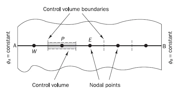
Grid Details:
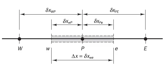
Discretised equation for 1D diffusion problem:
`int_(DeltaV) d/dx(Gamma (dphi)/dx) dV + int_(DeltaV) S dV = (Gamma A (dphi)/dx)_e - (Gamma A (dphi)/dx)_w + barS DeltaV = 0`
2) Major Differences between FDM and FVM:
| Sr. No. | Finite Difference Method (FDM) | Finite Volume Method (FVM) |
| 1 | Differential form of governing equation is used to formulate FDM | Integral form of the governing equation is used to formulate FVM |
| 2 | Computational Domain is discretised in the number of nodes where the parameters are evaluated. | Computational Domain is discretised in the number of control volumes over which the parameters are evaluated. Average values are stored at the nodes located at centroid of control volume. |
| 3 | Conservation of parameters is not ensured. | Conservation of parameters is ensured local level as well as global level |
| 4 | Can be used only for structured mesh. | Can be used for both structured as well as unstructured mesh. |
| 5 | Taylor series is used. | Divergence theorem is used. |
3)Necessity of interpolation schemes and different types of interpolation schemes:
The approximations of surface and volume integrals require values of the variables at the face centers while the average values are stored at cell centers (computational nodes). The values at face centers are interpolated from the neighbouring node values. Thus interpolation schemes are needed.
List of Interpolation Schemes:
(i) Linear Interpolation Scheme (Central Difference scheme)
(ii) Upwind Interpolation Scheme
(iii) Hybrid Interpolation Scheme
(iv) Quadratic Upwind interpolation scheme (QUICK)
(v) TVD schemes
(i) Linear Interpolation Scheme (Central Difference scheme):
In this scheme the variable values at faces are evaluated by using the linear interpolation of the values from the corresponding neighbouring nodes. It is second order accurate.
General formulation of Linear interpolation scheme is given as
`phi_e = phi_E.lamda_e + phi_P.(1- lamda_e)` where
`lamda_e = (x_e - x_P)/(x_E - x_P)`
For uniform grid face center values of variable `phi` in 1D problem are given as follows
`phi_e = (phi_P + phi_E)/2`
`phi_w = (phi_W + phi_P)/2`
It is simplest interpolation scheme so most widely used for approximation of diffusive fluxes.
It may produce oscillatory solutions with coarse grids so requires finer computational grids for stable solutions.
(ii) Upwind Interpolation Scheme:
The Upwind differencing scheme or 'donor cell' differencing scheme considers the direction of flow while evaluating the variable value at the face cell. So the convected value of the variable `phi` at the face center is taken to be equal to the value at the upstream computational node.
for 1D case
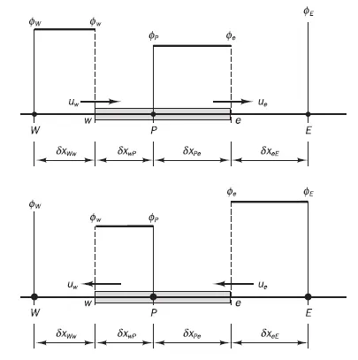
If flow is in positive x direction i.e. `u > 0 `
`phi_e = phi_P` and `phi_w = phi_W` .
Similarly if flow is in negative x direction i.e. `u < 0 `
`phi_e = phi_E` and `phi_w = phi_P` .
The Upwind interpolation scheme is the only interpolation scheme which is unconditionally bounded. Also as it considers the direction of flow the transportiveness is inherent.
It is first order accurate scheme thus the results include the artificial diffusion. The smearing out of sharp picks or rapid variations can be observed.
It needs very fine grid and grid alignment with flow direction for accurate solutions.
(iii) Hybrid Interpolation Scheme :
The hybrid interpolation scheme is the combination of the both linear interpolation scheme and upwind interpolation scheme. It exploits the favourable properties of linear interpolation and the upwind interpolation schemes based on the local Peclet number.
`phi_e = gamma.phi_(CDS) + (1- gamma).phi_(UDS)` where
`gamma` is evaluated using Local Peclet Number.
It produces physically realistic and highly stable solutions for 1D convection diffusion problem.
It is only first order accurate scheme.
(iv) Quadratic Upwind interpolation scheme (QUICK):
The Quadratic Upwind Interpolation for Convective Kinematics scheme makes use of three-point upstream-weighted quadratic interpolation to evaluate the variable value at the face center. The face center value of variable `phi` is obtained using two upstream nodes and one downstream node.
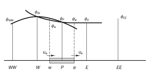
when `u_w >0 ` and `u_e >0` then
for evaluation of `phi_w` the node values from W, P and E are used while
for evaluation of `phi_e` the node values from P, E and EE are used.
Similarly when `u_w <0 ` and `u_e <0` then
for evaluation of `phi_w` the node values from P, W and WW are used while
for evaluation of `phi_e` the node values from E, P and W are used.
For uniform grid the general equation for value at face center is given as
`phi_(face) = 6/8 phi_U + 3/8 phi_D - 1/8 phi_(UU)`
where `D` denotes downstream node ,
`U` denotes neighbouring upstream node and
`UU` denotes an additional upstream node.
General Formulation of QUICK Scheme is as follows using `D, U "and" UU` notation is as follows
`phi_e = phi_U + g_1 (phi_D - phi_U) + g_2 (phi_(UU) - phi_U) ` where
`g_1 = ((x_e - x_U) (x_e - x_(UU)))/((x_D - x_U) (x_D - x_(UU)))` and `g_2 = ((x_e - x_U) (x_e - x_D))/((x_(UU) - x_U) (x_(UU) - x_D))` .
At the boundary nodes the required values are obtained using linear extrapolation and the mirror node for the evaluation of face center values as illustrated below
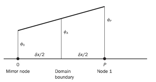
QUICK scheme gives more accurate results even for the coarse mesh.
It is conservative and third order accurate on both uniform and nonuniform grids.
It can give overshoots and undershoots in solution thus it is conditionally stable.
(v) Total Variation Diminishing (TVD) schemes:
The class of TVD schemes has been specially formulated to obtain oscillations free solutions and has proved to be useful in CFD calculations. In TVD schemes the tendency towards oscillations is counteracted by addition of artificial diffusion fragment or by adding a weighting towards upstream contributions.
General formulation of TVD scheme is given as
`phi_e = phi_P + 1/2 Psi(r) (phi_E - phi_P)` where ` r = ((phi_P - phi_W)/(phi_E - phi_P))`
and `Psi(r)` is known as `"Flux limiter function"` .
For above mentioned schemes, the face center value at face `e` can be expressed in terms of general TVD formulation as follows:
- For Upwind interpolation Scheme, `Psi(r) = 0` .
- For Linear interpolation Scheme (CDS), `Psi(r) = 1` .
- For QUICK Scheme , `Psi(r) = (3+r)/4` .
4) Necessity of `"Flux limiter function"` in FVM :
In order to make the scheme TVD, to constrain or to limit the range of possible values of the additional convective flux, `F_e Psi(r) (phi_E - phi_P)/2 ` which is originally introduce to make scheme higher order accurate. Thus the function `Psi(r)` is called as `"Flux limiter function"` .
The choice of the function `Psi(r)` determines the order of accuracy and boundedness of the scheme.