Week 3.5 - Deriving 4th order approximation of a 2nd order derivative using Taylor Table method

Aim: To Derive the 4th order approximations of the second-order derivative for
(i) Central difference scheme (Symmetric), (ii) Skewed right-sided difference scheme and (iii) Skewed left-sided differenc scheme using Taylor's Table Method and To test scheme for given function over the range of dx for absolute numerical error. To plot graph between absolute numerical error and `dx` .

Given: `f(x) = e^(x)*cos(x)` ;
`x= pi/3` over range of `dx` from `pi/4` to `pi/400` .

4th Order approximate second order numerical derivative using Central Difference (Symmetric) Scheme:

Number of nodes for Symmetric numerical stencil are calculated as follows:
`N= P + Q -1`

where -
`N - "Number of nodes to be considered"` ;
`P - "Order of Accuracy (or Order of approximation) required"` ;
`Q - "Order of derivative"`

hence, `N= 4 + 2 - 1= 5`.

Numerical Stencil is represented as :

`--ubrace(underset(i-2)(star)--underset(i-1)(star)--underset(i)(star)--underset(i+1)(star)--underset(i+2)(star)--)_("Numerical Stencil")`

`f''(x)~~ (delta^2f)/ (deltax^2)`

Hypothetical equation for cental difference scheme is given as
`f''(x)= (a*f(i-2)+b*f(i-1)+ c*f(i)+d*f(i+1)+e*f(i+2))/(Deltax^2) + O(Deltax^4)`

Taylor Table for Central Difference sheme is as follows:

`"Taylor Series Terms" rarr`	`f(i)`	`f^(i)(i)*Deltax`	`f^(ii)(i)*(Deltax^2)`	`f^(iii)(i)*(Deltax^3)`	`f^(iv) (i)*(Deltax^4)`
`a*f(i-2)`	`a`	`-2a`	`(4a)/2`	`(-8a)/6`	`(16a)/24`
`b*f(i-1)`	`b`	`-b`	`b/2`	`-b/6`	`b/24`
`c*f(i)`	`c`	`0`	`0`	`0`	`0`
`d*f(i+1)`	`d`	`d`	`d/2`	`d/6`	`d/24`
`e*f(i+2)`	`e`	`2e`	`(4e)/2`	`(8e)/6`	`(16e)/24`
Sum of Coeff Column equals to	`0`	`0`	`1`	`0`	`0`

From the Table the system of equations obtained is as follows:

`[[1,1,1,1,1],[-2,-1,0,1,2],[2,1/2,0,1/2,2],[(-4)/3,(-1)/6,0,1/6,4/6],[2/3,1/24,0,1/24,2/3]] [[a],[b],[c],[d],[e]] =[[0],[0],[1],[0],[0]]`

solving this system of equations we get ,

`[[a=(-1)/12],[b=4/3],[c=(-5)/2],[d=4/3],[e=(-1)/12]]`

Thus by Central Difference (Symmetric) scheme,

`f''(x) ~= ((-1/12)*f(i-2)+(4/3)*f(i-1)-(5/2)*f(i)+(4/3)*f(i+1)+(-1/12)*f(i+2))/(Deltax^2)`.

4th Order approximate second order numerical derivative using Skewed Right side Difference (Asymmetric) Scheme:

Number of nodes for Asymmetric numerical stencil are calculated as follows:
`N= P + Q`

where -
`N - "Number of nodes to be considered"` ;
`P - "Order of Accuracy (or Order of approximation) required"` ;
`Q - "Order of derivative"`

hence, `N= 4 + 2 = 6`.

Numerical Stencil is represented as :

`--ubrace(underset(i)(star)--underset(i+1)(star)--underset(i+2)(star)--underset(i+3)(star)--underset(i+4)(star)--underset(i+5)(star)--)_("Numerical Stencil")`

`f''(x)~~ (delta^2f)/ (deltax^2)`

Hypothetical equation for Skewed Right side difference scheme is given as
`f''(x)= (a*f(i)+b*f(i+1)+ c*f(i+2)+d*f(i+3)+e*f(i+4)+k*f(i+5))/(Deltax^2) + O(Deltax^4)`

Taylor Table for Skewed Right side Difference sheme is as follows:

`"Taylor Series Terms" rarr`	`f(i)`	`f^(i)(i)*Deltax`	`f^(ii)(i)*(Deltax^2)`	`f^(iii)(i)*(Deltax^3)`	`f^(iv) (i)*(Deltax^4)`	`f^v (i)*(Deltax^5)`
`a*f(i)`	`a`	`0`	`0`	`0`	`0`	`0`
`b*f(i+1)`	`b`	`b`	`b/2`	`b/6`	`b/24`	`b/120`
`c*f(i+2)`	`c`	`2c`	`(4c)/2`	`(8c)/6`	`(16c)/24`	`(32c)/120`
`d*f(i+3)`	`d`	`3d`	`(9d)/2`	`(27d)/6`	`(81d)/24`	`(243d)/120`
`e*f(i+4)`	`e`	`4e`	`(16e)/2`	`(64e)/6`	`(256e)/24`	`(1024e)/120`
`k*f(i+5)`	`k`	`5k`	`(25k)/2`	`(125k)/6`	`(625k)/24`	`(3125k)/120`
Sum of Coeff Column equals to	`0`	`0`	`1`	`0`	`0`	`0`

From the Table the system of equations obtained is as follows:

`[[1,1,1,1,1,1],[0,1,2,3,4,5],[0,1/2,2,9/2,8,25/2],[0,1/6,4/3,9/2,32/3,125/6],[0,1/24,2/3,27/8,32/3,625/24],[0,1/120,4/15,81/40,128/15,625/24]] [[a],[b],[c],[d],[e],[k]] =[[0],[0],[1],[0],[0],[0]]`

solving this system of equations we get ,

`[[a=15/4],[b=(-77)/6],[c=107/6],[d=(-13)],[e=61/12],[k=(-5)/6]]`

Thus by Skewed Right side Difference (Asymmetric) scheme,

`f''(x) ~= ((15/4)*f(i)-(77/6)*f(i+1)+(107/6)*f(i+2)-(13)*f(i+3)+(61/12)*f(i+4)-(5/6)*f(i+5))/(Deltax^2)`

4th Order approximate second order numerical derivative using Skewed Left side Difference (Asymmetric) Scheme:

Number of nodes for Asymmetric numerical stencil are calculated as follows:
`N= P + Q`

where -
`N - "Number of nodes to be considered"` ;
`P - "Order of Accuracy (or Order of approximation) required"` ;
`Q - "Order of derivative"`

hence, `N= 4 + 2 = 6`.

Numerical Stencil is represented as :

`--ubrace(underset(i-5)(star)--underset(i-4)(star)--underset(i-3)(star)--underset(i-2)(star)--underset(i-1)(star)--underset(i)(star)--)_("Numerical Stencil")`

`f''(x)~~ (delta^2f)/ (deltax^2)`

Hypothetical equation for Skewed Left side difference scheme is given as
`f''(x)= (a*f(i)+b*f(i-1)+ c*f(i-2)+d*f(i-3)+e*f(i-4)+k*f(i-5))/(Deltax^2) + O(Deltax^4)`

Taylor Table for Skewed Left side Difference sheme is as follows:

`"Taylor Series Terms" rarr`	`f(i)`	`f^(i)(i)*Deltax`	`f^(ii)(i)*(Deltax^2)`	`f^(iii)(i)*(Deltax^3)`	`f^(iv) (i)*(Deltax^4)`	`f^v (i)*(Deltax^5)`
`a*f(i)`	`a`	`0`	`0`	`0`	`0`	`0`
`b*f(i-1)`	`b`	`(-b)`	`b/2`	`(-b)/6`	`b/24`	`(-b)/120`
`c*f(i-2)`	`c`	`(-2c)`	`(4c)/2`	`(-8c)/6`	`(16c)/24`	`(-32c)/120`
`d*f(i-3)`	`d`	`(-3d)`	`(9d)/2`	`(-27d)/6`	`(81d)/24`	`(-243d)/120`
`e*f(i-4)`	`e`	`(-4e)`	`(16e)/2`	`(-64e)/6`	`(256e)/24`	`(-1024e)/120`
`k*f(i-5)`	`k`	`(-5k)`	`(25k)/2`	`(-125k)/6`	`(625k)/24`	`(-3125k)/120`
Sum of Coeff Column equals to	`0`	`0`	`1`	`0`	`0`	`0`

From the Table the system of equations obtained is as follows:

`[[1,1,1,1,1,1],[0,-1,-2,-3,-4,-5],[0,1/2,2,9/2,8,25/2],[0,(-1)/6,(-4)/3,(-9)/2,(-32)/3,(-125)/6],[0,1/24,2/3,27/8,32/3,625/24],[0,(-1)/120,(-4)/15,(-81)/40,(-128)/15,(-625)/24]] [[a],[b],[c],[d],[e],[k]] =[[0],[0],[1],[0],[0],[0]]`

solving this system of equations we get ,

`[[a=15/4],[b=(-77)/6],[c=107/6],[d=(-13)],[e=61/12],[k=(-5)/6]]`

Thus by Skewed Left side Difference (Asymmetric) scheme,

`f''(x) ~= ((15/4)*f(i)-(77/6)*f(i-1)+(107/6)*f(i-2)-(13)*f(i-3)+(61/12)*f(i-4)-(5/6)*f(i-5))/(Deltax^2)`

Functions are written in the MATLAB to solve system of equations for Central difference (symmetric) scheme , Skewed Right side difference (Asymmetric) scheme and Skewed Left side difference (Asymmetric) scheme.

Code for Scheme coefficients:

close all
clear all
clc

%Inputs for number of nodes, order of approximations and order of derivative
n=6;        % Number of nodes = order of approximation + order of derivative
d=2;        % Order of numerical derivative to be calculated
% Function call for Taylor table Coefficients Symmetric stencil and no of nodes for symmetric stencil
[a]= Taylor_table_coeff_symmetric_stencil((n-1),d); 

% Function call for Taylor table Coefficients right skewed stencil and no of nodes for skewed stencil
[b]= Taylor_table_coeff_right_skewed_stencil(n,d);

% Function call for Taylor table Coefficients left skewed stencil and no of nodes for skewed stencil
[c]= Taylor_table_coeff_left_skewed_stencil(n,d);

% Array of taylor table coeff for symmetric stencil a,b,c,d,e respectively 
Symmetric_stencil=a' 

% Array of taylor table coeff for Asymmetric right skewed stencil
% a,b,c,d,e,k respectively
Right_skewed_stencil=b'

% Array of taylor table coeff for Asymmetric left skewed stencil
% a,b,c,d,e,k respectively
Left_skewed_stencil=c'

function code: Taylor_table_coeff_symmetric_stencil.m

function [a]=Taylor_table_coeff_symmetric_stencil(n,d)    
A=zeros(n);
         for i=1:n
               m = -(n-1)/2;
               for j=1:n  
                 A(i,j)= ((-1).*(-m)).^(i-1)/factorial(i-1);
                m= m+1;    
               end
         end
X=A^-1;
[a]=X(:,(d+1));
end

function code: Taylor_table_coeff_right_skewed_stencil.m

function [a]=Taylor_table_coeff_right_skewed_stencil(n,d)
    A=zeros(n);
         for i=1:n
               for j=1:n  
                 A(i,j)= (j-1).^(i-1)/factorial(i-1);    
               end
         end
X=A^-1;
[a]=X(:,(d+1));
end

function code: Taylor_table_coeff_left_skewed_stencil.m

function [a]=Taylor_table_coeff_left_skewed_stencil(n,d)
    A=zeros(n);
         for i=1:n
               for j=1:n  
                 A(i,j)= (1-j).^(i-1)/factorial(i-1);    
               end
         end
X=A^-1;
[a]=X(:,(d+1));
end

Output:

Symmetric_stencil =

   -0.0833    1.3333   -2.5000    1.3333   -0.0833


Right_skewed_stencil =

    3.7500  -12.8333   17.8333  -13.0000    5.0833   -0.8333


Left_skewed_stencil =

    3.7500  -12.8333   17.8333  -13.0000    5.0833   -0.8333

MATLAB code has been written to compule Exact second order derivative of function `f(x) = e^(x)*cos(x)`
i.e. `f''(x)=-2*e^(x)*sin(x)` at `x=pi/3` over the range of `dx` from `pi/4` to `pi/400` and 4th order approximate second order numerical derivatives using schemes developed earlier.

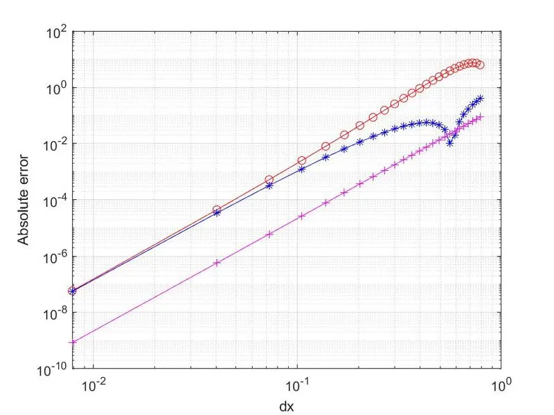
The Absolute Numerical error is calculated for each perticular value of `dx` and logarithmic plot of `" Absolute Numerical Error"` against `dx` and conclusins are drawn on trends of graph.

Main code:

close all
clear all
clc

% Given Function is f(x)=exp(x)*cos(x)

% values of x and dx
x=pi/3;
dx=linspace(pi/400,pi/4,25);

% Analytical second order Derivative of f(x)= f''(x)=(-2).*exp(x).*sin(x)
Analytical_second_order_Derivative =(-2).*exp(x).*sin(x);

    Num_2nd_deri_4th_order_approx_right_skewed=zeros(1,length(dx));
    Num_2nd_deri_4th_order_approx_left_skewed=zeros(1,length(dx));
    Num_2nd_deri_4th_order_approx_symmetric=zeros(1,length(dx));
    
    
    Error_4th_order_right_skewed=zeros(1,length(dx));
    Error_4th_order_left_skewed=zeros(1,length(dx));
    Error_4th_order_symmetric=zeros(1,length(dx));
 

for i=1:length(dx)
    % Second order Numerical Derivative by Right skewed scheme
    Num_2nd_deri_4th_order_approx_right_skewed(i) = (((15/4).*exp(x).*cos(x))+((-77/6).*exp(x+dx(i)).*cos(x+dx(i)))+((107/6).*exp(x+(2*dx(i))).*cos(x+(2*dx(i))))+((-13).*exp(x+(3*dx(i))).*cos(x+(3*dx(i))))+((61/12).*exp(x+(4*dx(i))).*cos(x+(4*dx(i))))+((-5/6).*exp(x+(5*dx(i))).*cos(x+(5*dx(i)))))/(dx(i).^2);
   
    % Second order Numerical Derivative by Left skewed scheme 
    Num_2nd_deri_4th_order_approx_left_skewed(i) = (((15/4).*exp(x).*cos(x))+((-77/6).*exp(x-dx(i)).*cos(x-dx(i)))+((107/6).*exp(x-(2*dx(i))).*cos(x-(2*dx(i))))+((-13).*exp(x-(3*dx(i))).*cos(x-(3*dx(i))))+((61/12).*exp(x-(4*dx(i))).*cos(x-(4*dx(i))))+((-5/6).*exp(x-(5*dx(i))).*cos(x-(5*dx(i)))))/(dx(i).^2);
    
    % Second order Numerical Derivative by Symmetric scheme
    Num_2nd_deri_4th_order_approx_symmetric(i) = (((-1/12).*exp(x-(2*dx(i))).*cos(x-(2*dx(i))))+((4/3).*exp(x-dx(i)).*cos(x-dx(i)))+((-5/2).*exp(x).*cos(x))+((4/3).*exp(x+dx(i)).*cos(x+dx(i)))+((-1/12).*exp(x+(2*dx(i))).*cos(x+(2*dx(i)))))/(dx(i).^2);
    
    % error patameter = err = abs(Exact derivative at pi/3 - Numerical derivative at pi/3)

    Error_4th_order_right_skewed(i) = abs(Analytical_second_order_Derivative - Num_2nd_deri_4th_order_approx_right_skewed(i));

    Error_4th_order_left_skewed(i) = abs(Analytical_second_order_Derivative - Num_2nd_deri_4th_order_approx_left_skewed(i));

    Error_4th_order_symmetric(i) = abs(Analytical_second_order_Derivative - Num_2nd_deri_4th_order_approx_symmetric(i));

    
end

a=dx;
b=[Error_4th_order_right_skewed ; Error_4th_order_left_skewed ;Error_4th_order_symmetric];

figure(1)
loglog(a,b(1,:),'r-o',a,b(2,:),'b-*',a,b(3,:),'m-+')
xlabel('dx')
ylabel('Absolute error')
grid on
grid minor

saveas(gcf,'4th order Loglog graph','jpg')

Logarithmic Plot:

Conclusions:

1. From the graph it is clear that the order of convergence of Central Difference (symmetric) scheme is higher than order of convergenve of the Skewed Right Side difference and Skewed Left side difference (Assymetric) schemes.
2. For higher values of `dx` the difference between the absolute numerical errors of Skewed Right side Difference Scheme and Skewed Left side Difference Scheme is higher as values of `dx` gets smaller the difference between the absolute numerical errors mitigates.
3. For Higher values of `dx`the absolute numerical error oscillates for certain range of `dx`but stabilises further for lesser values od `dx`

Importance of Skewed (Asymmetric) Schemes:

Though Central difference (symmetric) scheme converges faster than the Skewed Schemes but it cannot be implemented on the boundaries due to unavailability of nodes on one side thus, on the boundaries the skewed difference schemes are implemented.