Week 11 - Simulation of Flow through a pipe in OpenFoam

 Aim:

1. To simulate the flow through pipe using axis symmetry by applying wedge boundary     
   conditions in OpenFOAM. Consider the flow to be laminar with Reynolds number 2100 for any diameter of the pipe.  Compare the results with Hagen-Poiseuille's equations for flow through circular pipe.
   Expected Results:
   • Validation of hydrodynamic length with Numerical results.
   • Validation of velocity profile of fully developed flow with its analytical profile.
   • Validation of max velocity and pressure drop for fully developed flow.
   • Post processing of shear stress and validation of wall shear stress for fully developed flow.   
2. To write a MATLAB code for automatic generation of fully functional the blockMeshDict file for  given input parameters.

Parameters:

1. Radius of Pipe (`R`) `= 0.0075 "m"`   i.e. `D=0.015 m`  .
2. Reynolds number (`Re`) `= 2100`  .
3. Dynamic Viscosity (`mu`) of water `= 0.001 Pa-s` .
4. Density of water (`rho`) = `1000 "kg"/m^3` .   

Calculations:

The calculations are based on the Hagen Poiseuille's equation for flow through circular pipe, which are as follows: 

1. Hydrodynamic entrance length (`Le`) `= 0.06*"Re"*D =1.89 m`  .
2. Length of pipe (`L`) `= Le +0.5 = 2.39 m` .
3. Average flow velocity using `Re` , `V_"avg" = (mu*"Re")/(rho*D) = 0.14 m/s`  .
4. Friction factor for Laminar flow (`f`) `= 64/"Re" = 0.0305 ` .
5. Pressure gradient (`- (delP)/(delx)`) `= (f*rho*(V_"avg")^2)/(2*D) = 19.91 N/m^3`
6. Maximum velocity (`V_"max"`) `= 2 * V_"avg" = 0.28 m/s` . 
7. Max Shear stress occurs at wall (`tau_"wall"`) `= 8*mu*V_"avg"/D = 0.0747 N/m^2` .
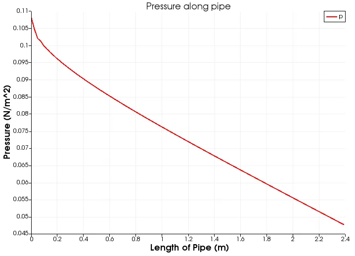
8. Dynamic Pressure drop at outlet (`DeltaP`) `= (- (delP)/(delx))*"Le"/rho =0.0476 m^2/s^2` .
9. Radial velocity profile is given by `V_r = (1/(4mu))(- (delP)/(delx))*(R^2 -r^2)`
   where `r `- radial distance (`m`) .

Workflow:

(1) MATLAB code for automatic generation of fully functional the blockMeshDict file with necessary input parameters.

close all
clear all
clc

% input parameters
theta = 2;                                 % halfangle of wedge in degrees
radius = 0.0075;                           % radius of pipe in m 
Re = 2100 ;                                % Reynolds number
hydlength = 0.06*Re*2*radius ;             % Hydrodynamic Entrance length
length = hydlength + 0.5;                 % Pipe length
p1 = radius*cosd(theta);                   % calculation for point 1
p2 = radius*sind(theta);                   % calculation for point 2 

% Vertex inputs
xmin= 0;                          
xmax= length;
ymin= 0;
ymax= p1; 
zmax= p2; 
zmin=-1.0*p2;

% Mesh gridpoints and simple grading inputs

nx = 50;
ny = 1;
nz = 100;
gx = 0.1;
gy = 1;
gz = 1;

%% Writing blockMeshDict file

f1=fopen('blockMeshDict.txt','w');
fprintf(f1,'\n/*--------------------------------*- C++ -*----------------------------------*\\');
fprintf(f1,'\n  =========                 |');
fprintf(f1,'\n  \\      /  F ield         | OpenFOAM: The Open Source CFD Toolbox ');
fprintf(f1,'\n   \\    /   O peration     | Website:  https://openfoam.org ');
fprintf(f1,'\n    \\  /    A nd           | Version:  9 ');
fprintf(f1,'\n     \\/     M anipulation  |\n');
fprintf(f1,'\n\\*---------------------------------------------------------------------------*/');
fprintf(f1,'\nFoamFile \n {\n    format      ascii;\n    class       dictionary;\n    object      blockMeshDict;\n  }');
fprintf(f1,'\n// * * * * * * * * * * * * * * * * * * * * * * * * * * * * * * * * * * * * * //');
fprintf(f1,'\n\nconvertToMeters 1;\n');
fprintf(f1,'\nvertices\n(\n    (%f %f %f)       //0 \n',xmin,ymin,ymin);
fprintf(f1,'    (%f %f %f)       //1 \n',xmin,ymax,zmax);
fprintf(f1,'    (%f %f %f)       //2 \n',xmin,ymax,zmin);
fprintf(f1,'    (%f %f %f)       //3 \n',xmax,ymin,ymin);
fprintf(f1,'    (%f %f %f)       //4 \n',xmax,ymax,zmax);
fprintf(f1,'    (%f %f %f)       //5 \n\n  );\n',xmax,ymax,zmin);
fprintf(f1,'blocks \n(\n     hex (0 2 1 0 3 5 4 3) (%d %d %d) simpleGrading (%f %f %f) \n\n  );\n',nx,ny,nz,gx,gy,gz);
fprintf(f1,'edges \n (\n     arc 1 2 (%f %f %f) \n     arc 4 5 (%f %f %f) \n  );\n',xmin,radius,0,xmax,radius,0);
fprintf(f1,'boundary \n(\n    inlet \n     {\n        type patch; \n        faces \n        (\n             (0 1 2 0) \n        );\n    }\n');
fprintf(f1,'    outlet \n    {\n        type patch; \n        faces \n        ( \n            (3 4 5 3) \n        ); \n    }\n');
fprintf(f1,'    upperWall \n    {\n        type wall; \n        faces \n        (\n            (2 1 5 4) \n       ); \n    }\n');
fprintf(f1,'    front \n    {\n        type wedge; \n        faces \n        (\n            (0 3 4 1) \n        ); \n    }\n');
fprintf(f1,'    back \n    {\n        type wedge; \n        faces \n        (\n            (0 2 5 3) \n         ); \n    }\n);\n');
fprintf(f1,'// ************************************************************************* //');   
fclose(f1);

Ouput: Fully functional blockMeshDict file

/*--------------------------------*- C++ -*----------------------------------*\
  =========                 |
  \      /  F ield         | OpenFOAM: The Open Source CFD Toolbox 
   \    /   O peration     | Website:  https://openfoam.org 
    \  /    A nd           | Version:  9 
     \/     M anipulation  |

\*---------------------------------------------------------------------------*/
FoamFile 
 {
    format      ascii;
    class       dictionary;
    object      blockMeshDict;
  }
// * * * * * * * * * * * * * * * * * * * * * * * * * * * * * * * * * * * * * //

convertToMeters 1;

vertices
(
    (0.000000 0.000000 0.000000)       //0 
    (0.000000 0.007495 0.000262)       //1 
    (0.000000 0.007495 -0.000262)       //2 
    (2.390000 0.000000 0.000000)       //3 
    (2.390000 0.007495 0.000262)       //4 
    (2.390000 0.007495 -0.000262)       //5 

  );
blocks 
(
     hex (0 2 1 0 3 5 4 3) (50 1 100) simpleGrading (0.100000 1.000000 1.000000) 

  );
edges 
 (
     arc 1 2 (0.000000 0.007500 0.000000) 
     arc 4 5 (2.390000 0.007500 0.000000) 
  );
boundary 
(
    inlet 
     {
        type patch; 
        faces 
        (
             (0 1 2 0) 
        );
    }
    outlet 
    {
        type patch; 
        faces 
        ( 
            (3 4 5 3) 
        ); 
    }
    upperWall 
    {
        type wall; 
        faces 
        (
            (2 1 5 4) 
       ); 
    }
    front 
    {
        type wedge; 
        faces 
        (
            (0 3 4 1) 
        ); 
    }
    back 
    {
        type wedge; 
        faces 
        (
            (0 2 5 3) 
         ); 
    }
);
// ************************************************************************* //

(2) OpenFOAM case set up:

     BlockMeshDict file is as generated above.

     Initial Velocity boundary conditions (U file in 0 folder):

/*--------------------------------*- C++ -*----------------------------------*\
  =========                 |
  \\      /  F ield         | OpenFOAM: The Open Source CFD Toolbox
   \\    /   O peration     | Website:  https://openfoam.org
    \\  /    A nd           | Version:  9
     \\/     M anipulation  |
\*---------------------------------------------------------------------------*/
FoamFile
{
    format      ascii;
    class       volVectorField;
    object      U;
}
// * * * * * * * * * * * * * * * * * * * * * * * * * * * * * * * * * * * * * //

dimensions      [0 1 -1 0 0 0 0];

internalField   uniform (0 0 0);

boundaryField
{
    inlet
    {
        type            fixedValue;
        value           uniform (0.14028 0 0);
    }

    outlet
    {
        type            zeroGradient;
    }

    upperWall
    {
        type            noSlip;
    }

    front
    {
        type            wedge;
    }

    back
    {
        type            wedge;
    }
}

// ************************************************************************* //

Initial pressure boundary conditions (p file in 0 folder):

/*--------------------------------*- C++ -*----------------------------------*\
  =========                 |
  \\      /  F ield         | OpenFOAM: The Open Source CFD Toolbox
   \\    /   O peration     | Website:  https://openfoam.org
    \\  /    A nd           | Version:  9
     \\/     M anipulation  |
\*---------------------------------------------------------------------------*/
FoamFile
{
    format      ascii;
    class       volScalarField;
    object      p;
}
// * * * * * * * * * * * * * * * * * * * * * * * * * * * * * * * * * * * * * //

dimensions      [0 2 -2 0 0 0 0];

internalField   uniform 0;

boundaryField
{
   inlet
    {
        type            zeroGradient;
    }

    outlet
    {
        type            fixedValue;
        value           uniform 0.047683;
    }
    
    upperWall
    {
        type zeroGradient;
       
    }
    
    front
    {
        type wedge;
       
    }
     
    back
    {
        type wedge;
     }

    
}

// ************************************************************************* //

Thermophysical properties (Transportproperties file from constant folder):

/*--------------------------------*- C++ -*----------------------------------*\
  =========                 |
  \\      /  F ield         | OpenFOAM: The Open Source CFD Toolbox
   \\    /   O peration     | Website:  https://openfoam.org
    \\  /    A nd           | Version:  9
     \\/     M anipulation  |
\*---------------------------------------------------------------------------*/
FoamFile
{
    format      ascii;
    class       dictionary;
    location    "constant";
    object      transportProperties;
}
// * * * * * * * * * * * * * * * * * * * * * * * * * * * * * * * * * * * * * //

transportModel  Newtonian;

nu              [0 2 -1 0 0 0 0] 1e-06;

// ************************************************************************* //

Solution controls (controlDict file from system folder):

/*--------------------------------*- C++ -*----------------------------------*\
  =========                 |
  \\      /  F ield         | OpenFOAM: The Open Source CFD Toolbox
   \\    /   O peration     | Website:  https://openfoam.org
    \\  /    A nd           | Version:  9
     \\/     M anipulation  |
\*---------------------------------------------------------------------------*/
FoamFile
{
    format      ascii;
    class       dictionary;
    location    "system";
    object      controlDict;
}
// * * * * * * * * * * * * * * * * * * * * * * * * * * * * * * * * * * * * * //

application     icoFoam;

startFrom       startTime;

startTime       0;

stopAt          endTime;

endTime         15;

deltaT          0.01;

writeControl    timeStep;

writeInterval   100;

purgeWrite      0;

writeFormat     ascii;

writePrecision  6;

writeCompression off;

timeFormat      general;

timePrecision   6;

runTimeModifiable true;


// ************************************************************************* //

Mesh is generated using blockMesh command and it has been checked by checkMesh command. Mesh quality is found to be OK. Mesh has also been inspected in paraview using paraFoam command.

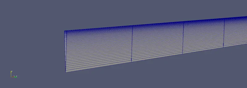
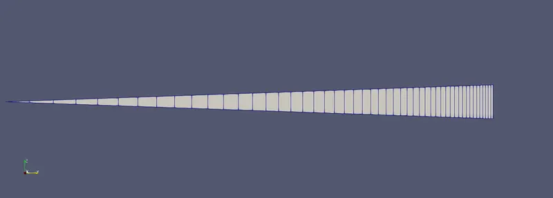
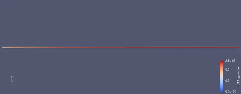
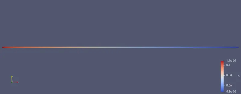
 Simulation is done bu using icoFoam command and results are obtained. Same are post processed in the paraview using paraFoam command. As we simulated the pipe flow for the small sector of pipe with wedge of angle `4^@` , to obtain the results for full cross section of pipe the reflect filter from paraview is used. Then using slice command the diametric place from the geometry is obtained to do further post processing. The velocity and pressure contours for various time steps are observed found accetable with the analytical results from Hagen Poiseuille's equations.

Velocity contour over full length of pipe:

Pressure contour over full length of pipe:

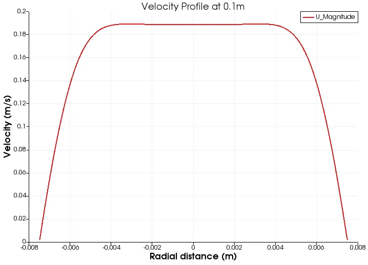
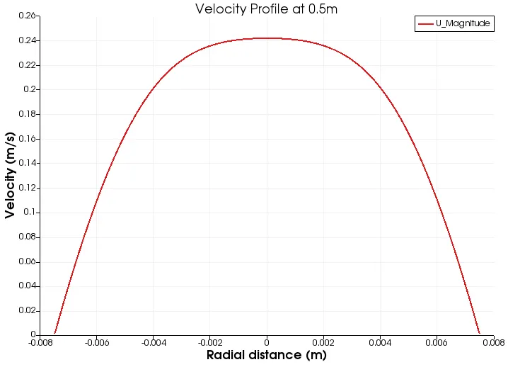
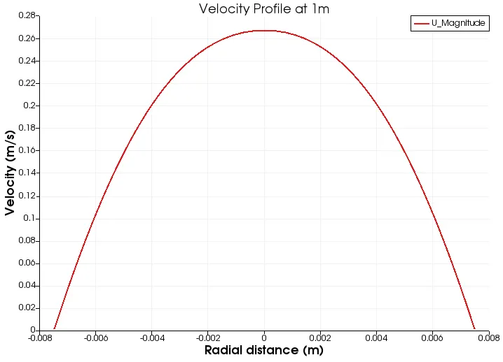
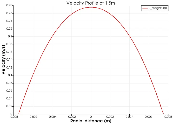
Velocity profiles are inspected at different lengths over cross section of pipe :

  (i) Velocity Profile at 0.1 m from inlet:

(ii) Velocity Profile at 0.5 m from inlet:

(iii) Velocity Profile at 1 m from inlet:

(iv) Velocity Profile at 1.5 m from inlet:

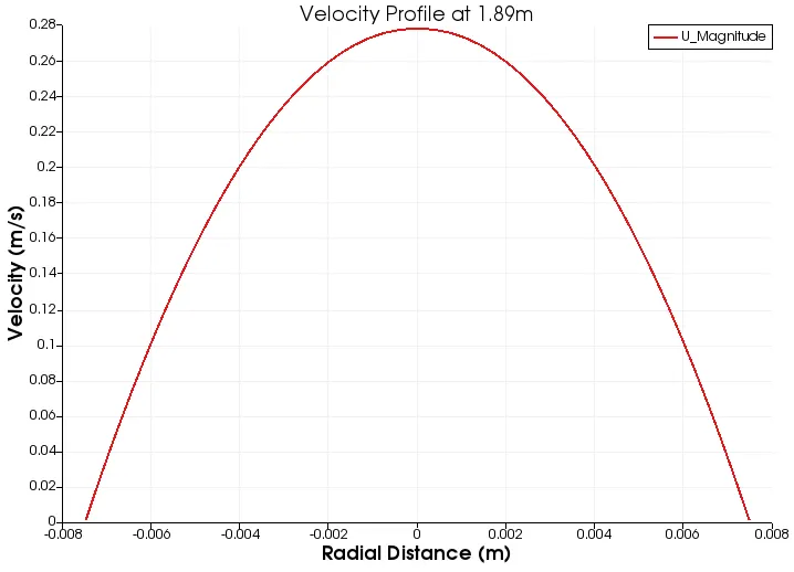
(v) Velocity Profile at 1.89 m from inlet:

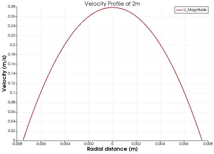
(vi) Velocity Profile at 2 m from inlet:

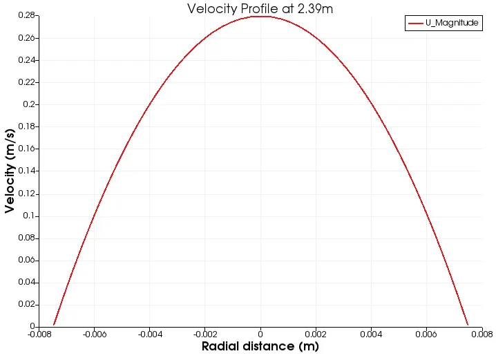
(i) Velocity Profile at 2.39 m from inlet (at outlet):

The Pressure over the entire length of pipe is also obtained using line over plot filter. The graph is as follows:

As shear stress is not a primitive variable that has to be obtained through calculations of primitive variables as follows:

(i) First of all using calculator filter the magnitude of velocity (Mag_U) is obtained for entire domain.

(ii) Then gradient of magnitude of velocity (Grad_Mag_U) is obtained using filter gradient of unstructured dataset.

(iii) As as shear stress (Tau) is gradient of velocity is coefficient of viscosity times gradient of velocity. It is obtained using calculator filter.

(iv) As shear stress is tensor its magnitude (Mag_Tau) is obtained using calculator filter. 

(v) The shear stress profile are obtained at the distance of 1.89m from the inlet. The graph is as follows:

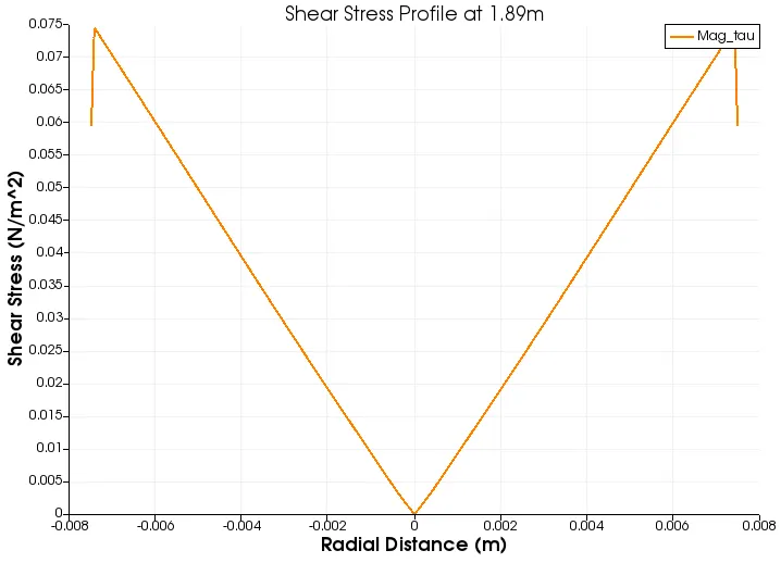
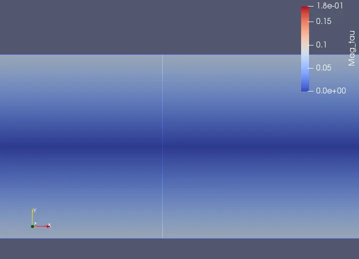
After this, the required data from the results at the distance of 1.89 m from inlet are obtained through paraview using spreadsheet view (CSV file and text files are attached herewith). The same data is used in MATLAB by file parsing technique and the result data is comapared with analytical data by using following MATLAB code.

close all
clear all
clc
 
%% Inputs for Analytical solution of Hagen Poiseuille
theta = 2;                                 % halfangle of wedge in degrees
radius = 0.0075;                           % radius of pipe in m 
Re = 2100 ;                                % Reynolds number
hydlength = 0.06*Re*2*radius ;             % Hydrodynamic Entrance length
length = hydlength + 0.5;                  % Pipe length
mu=0.001;                                  % Dynamic viscosity of water
rho=1000;                                  % Desity of water 
f=64/Re;                                   % Friction factor for laminar flow 
Vavg=Re*mu/(rho*2*radius);                 % Avg velocity computation using Re number 

y =linspace(0,radius,1000);                        % Radial distance
V =(0.0625*f*rho*Vavg^2/(radius*mu))*(radius^2-y.^2); % Velocity profile
Vmax =(0.0625*f*rho*Vavg^2/(radius*mu))*(radius^2);   % Max velocity
tau =(0.125*f*rho*Vavg^2/radius)*y;                % Shear stress
deltap_l =(0.25*f*rho*Vavg^2/radius);              % Pressure gradient per unit length
tau_max =max(tau);                                 % Calculated max shear stress
DeltaP_o =deltap_l*(2.39)/rho;                     % Dynamic pressure diffence at outlet

%% Data Reading from Paraview data file and data plotting
f1=fopen('data.txt','r');
fgetl(f1)
A=fscanf(f1,'%f',[3 inf]);
A=A';
fclose(f1);
figure(1)
Vmaximum=max(A(:,2));               % Maximum velocity from result data
tau_maximum=max(A(:,3));            % Maximum shear stress from result data

plot(A(:,2),A(:,1),'b',LineWidth=2)
grid on
grid minor
hold on
plot(V,y,'r',LineWidth=2)
hold on
plot(V,-y,'r',LineWidth=2)
title('Velocity Profile Comparison')
xlabel('Velocity (m/s)')
ylabel('Radial distance (m)')
legend ('Computional Velocity','Analytical Velocity')
saveas(gcf,'Velocity Profile study','png')


figure(2)
plot(A(:,3),A(:,1),'b',LineWidth=2)
grid on
grid minor
hold on
plot(tau,y,'r',LineWidth=2)
hold on
plot(tau,-y,'r',LineWidth=2)
title('Shear stress Profile Comparison')
xlabel('Shear stress (N/m^2)')
ylabel('Radial distance (m)')
legend ('Computional Shear stress','Analytical Shear stress',Location='east') 
saveas(gcf,'Shear stress Profiles study','png')

Workspace screenshot:

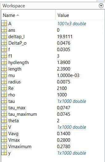
Velocity Profile Comparison:

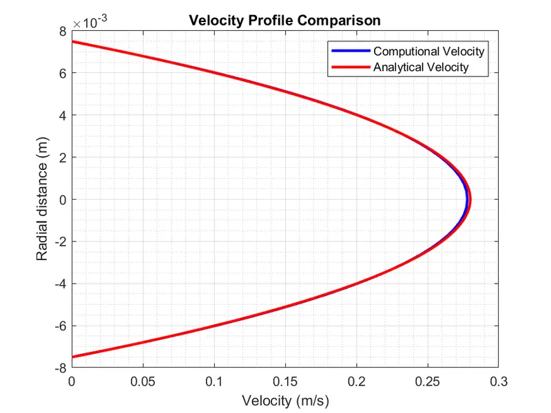
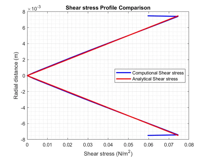
Shear stress profile comparison:

Observations and Conclusions:

1. Analytical hydrodynamic entrance length is validated with numerical results by comparing observing the velocity profiles at varoius locations along the pipe, from the velocity profiles it can be observed that the velocity profile is fully parabolic in nature with max velocity close to 0.28 m/s at the distance of 1.89 m from inlet.
2. Numerical Velocity profile is compared with Analytical velocity profile and the result are stated in velocity profile comparision. Close match of the velocity indicates that the numerical results are very close to analytical solution.
3. Numerical Values of `V_"max"` and `DeltaP` are extracted from data and found very close to the analytical values for `V_"max"` and `DeltaP`. Same can be observed at the screenshot of MATLAB workspace where the analytical and numerical results are compared.
4. Numerical value for wall shear stress (`tau_"wall"`) is post processed and found very close to analytical value. Also the numerical shear stress profile over cross section of pipe is compared with analytical shear stress profile, found similar and results are represented in the graph of shear stress profile comparision.
5. Thus the Hagen Poiseuille's equations for circular pipe are verified through numerical simulation of laminar flow through pipe.