Week 5.1 - Mid term project - Solving the steady and unsteady 2D heat conduction problem

Aim: To do steady state and transient state analysis for the 2D heat conduction problem with given boundary conditions using point iterative methods like Jacobi, Gauss Seidel and Successive Overrelaxation.

Given:

*Square domain with size `1 m` x `1 m` .

*Boundary conditions

Temperature at Left Boundary= `400 K`,

Temperature at Top Boundary= `600 K`,

Temperature at Right Boundary= `800 K`,

Temperature at Bottom Boundary= `900 K`.

Theory:

The general 2D heat conduction equation in cartesian coordinate system is given as follows:

`(delT)/(delt)=alpha((del^2T)/(delx^2) + (del^2T)/(dely^2) )` . It is an unsteady state 2D heat conduction PDE.

Steady state by definition does not include time derivative term hence steady state 2D heat conduction PDE becomes

`(del^2T)/(delx^2) + (del^2T)/(dely^2) =0`

Steady State Analysis:

The discretized form of steady state 2D heat conduction PDE using Central Difference Scheme for spatial terms is given by

`((T_(i-1,j) -2T_(i,j) +T_(i+1,j))/(Deltax^2)) + ((T_(i,j-1) -2T_(i,j) +T_(i,j+1))/(Deltay^2)) =0`

which on simplifying gives expression for node temperature `T_(i,j)` as

` T_(i,j) = ((Deltay^2)/(Deltax^2+Deltay^2))*((T_(i-1,j)+T_(i+1,j))/2) + ((Deltax^2)/(Deltax^2+Deltay^2))*((T_(i,j-1)+T_(i,j+1))/2)`

For Steady state analysis using Jacobi method the node temperature `T_(i,j)` is given as

` (T^(k+1))_(i,j) = ((Deltay^2)/(Deltax^2+Deltay^2))*(((T^k)_(i-1,j)+(T^k)_(i+1,j))/2) + ((Deltax^2)/(Deltax^2+Deltay^2))*(((T^k)_(i,j-1)+(T^k)_(i,j+1))/2)`

where `k` is the iteration number (generation of iteration).

For Steady state analysis using Gauss Seidel method the node temperature `T_(i,j)` is given as

` (T^(k+1))_(i,j) = ((Deltay^2)/(Deltax^2+Deltay^2))*(((T^(k+1))_(i-1,j)+(T^k)_(i+1,j))/2) + ((Deltax^2)/(Deltax^2+Deltay^2))*(((T^(k+1))_(i,j-1)+(T^k)_(i,j+1))/2)`

where `k` is the iteration number (generation of iteration).

For Steady state analysis using Successive Overrelaxation method the node temperature `T_(i,j)` is given as

` (T^(k+1))_(i,j) =(1-omega)*(T^(k))_(i,j) + omega*[((Deltay^2)/(Deltax^2+Deltay^2))*(((T^(k+1))_(i-1,j)+(T^k)_(i+1,j))/2) + ((Deltax^2)/(Deltax^2+Deltay^2))*(((T^(k+1))_(i,j-1)+(T^k)_(i,j+1))/2)]`

where `k` is the iteration number (generation of iteration) and `omega` is the relaxation factor .

Using above mentioned node temperature equations for respective iterative solver techniques the 2D heat conduction PDE is numerically solved till the convergence criterion is attained.

Unsteady/Transient State Analysis:

The discretized form of unsteady state 2D heat conduction PDE using Central Difference Scheme for spatial terms and first order forward difference scheme for time steps, is given by

`((T^(n+1))_(i,j) - (T^n)_(i,j))/(Deltat)=alpha*[((T_(i-1,j) -2T_(i,j) +T_(i+1,j))/(Deltax^2))^(n "or" (n+1)) + ((T_(i,j-1) -2T_(i,j) +T_(i,j+1))/(Deltay^2))^(n "or" (n+1))]`

where `n` is the `"time step" ` number and `alpha` is the `"Thermal Diffusivity"` .

According to the use of nth or (n+1)th time step temperature terms on RHS the The Unsteady state Analysis is divided into two categories i.e.

a) When nth time step temperature terms are used on RHS then it is known as Unsteady state Explicit method, The node temperature for (n+1)th time step `(T^(n+1))_(i,j)`

for explicit method after rearranging the above unsteady state discretized equation is given as

`(T^(n+1))_(i,j) = [1-((2alphaDeltat)/(Deltax^2))-((2alphaDeltat)/(Deltay^2))]*(T^n)_(i,j)+[(alphaDeltat)/(Deltax^2)]*[(T^n)_(i-1,j)+(T^n)_(i+1,j)] +[(alphaDeltat)/(Deltay^2)]*[(T^n)_(i,j-1)+(T^n)_(i,j+1)]`

In this case as `(T^(n+1))_(i,j)`

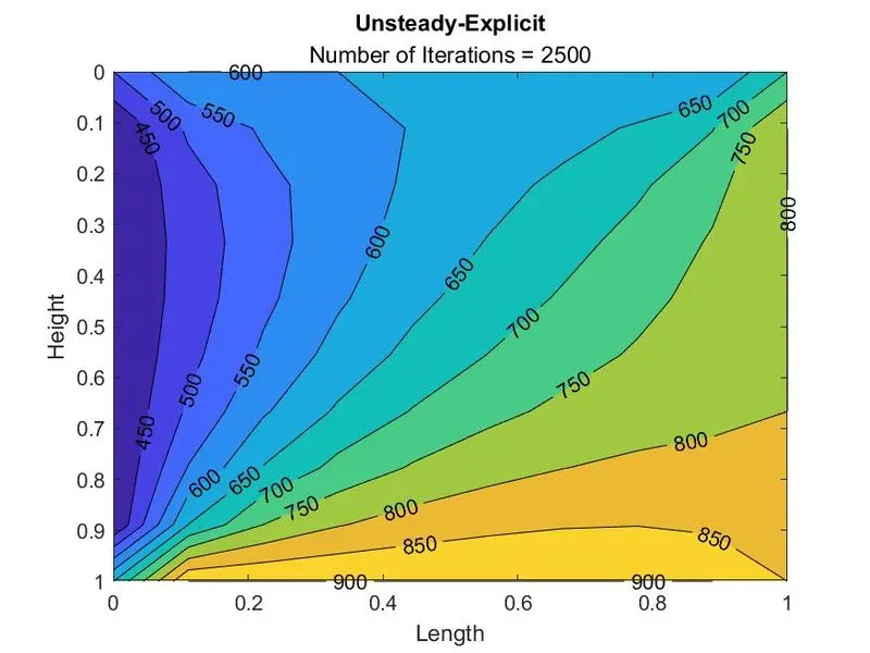
is directectly expressed in the all known terms thus it gives the direct numerical value of node temperature for next time step. Thus for the solution to converge it requires a large number of time steps.

b) When (n+1)th time step temperature terms are used on RHS then it is known as Unsteady state Implicit method.

The node temperature `(T^(n+1))_(i,j)`

for Unsteady state Implicit Jacobi method after rearranging the above unsteady state discretized equation is given as

`(T^(n+1))_(i,j) = [1+((2alphaDeltat)/(Deltax^2))+((2alphaDeltat)/(Deltay^2))]^(-1)*[(T^n)_(i,j)+[(alphaDeltat)/(Deltax^2)]*[(Told^(n+1))_(i-1,j)+(Told^(n+1))_(i+1,j)] +(alphaDeltat)/(Deltay^2)]*[(Told^(n+1))_(i,j-1)+(Told^(n+1))_(i,j+1)]`

The node temperature `(T^(n+1))_(i,j)`

for Unsteady state Implicit Gauss Seidel method after rearranging the above unsteady state discretized equation is given as

`(T^(n+1))_(i,j) = [1+((2alphaDeltat)/(Deltax^2))+((2alphaDeltat)/(Deltay^2))]^(-1)*[(T^n)_(i,j)+[(alphaDeltat)/(Deltax^2)]*[(T^(n+1))_(i-1,j)+(Told^(n+1))_(i+1,j)] +[(alphaDeltat)/(Deltay^2)]*[(T^(n+1))_(i,j-1)+(Told^(n+1))_(i,j+1)]`

The node temperature `(T^(n+1))_(i,j)`

for Unsteady state Implicit Successive Overrelaxation method after rearranging the above unsteady state discretized equation is given as

`(T^(n+1))_(i,j) = (1-omega)*(Told^(n+1))_(i,j) + omega*[[1+((2alphaDeltat)/(Deltax^2))+((2alphaDeltat)/(Deltay^2))]^(-1)*[(T^n)_(i,j)+[(alphaDeltat)/(Deltax^2)]*[(T^(n+1))_(i-1,j)+(Told^(n+1))_(i+1,j)] +[(alphaDeltat)/(Deltay^2)]*[(T^(n+1))_(i,j-1)+(Told^(n+1))_(i,j+1)]]`

where `alpha` is `"Thermal Diffusivity"` and `omega` is the relaxation factor.

Workflow:

1) The main code is written using functions for each method.

2) Each method is recalled using functions with necessary inputs and required outputs are defined.

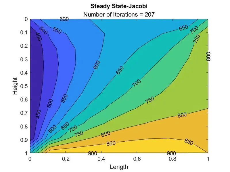
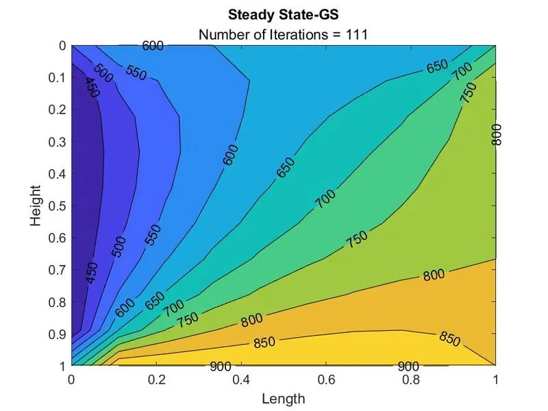
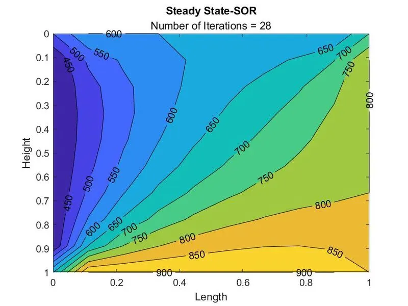
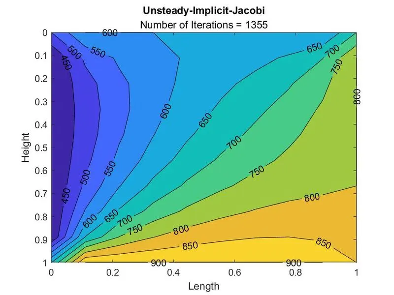
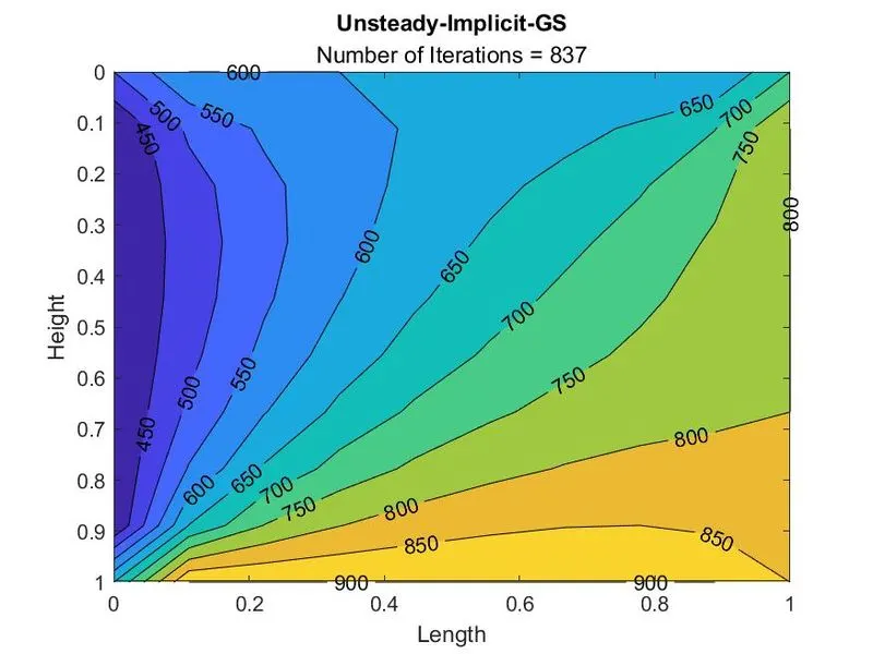
3) Temperature contour is saved for each method separately. Number of iterations shown on the plot title.

4) Compared the results and conclusions are drawn.

Main Code:

%Code to solve a second order 2 dimensional pde
% (d^2T/dx^2)+(d^2T/dy^2)=0 - Steady state
% alpha*((d^2T/dx^2)+(d^2T/dy^2))=dT/dt - Unsteady/Transient state

clear all
close all
clc

%inputs
L=1;                       % Domain Length
H=1;                       % Domain Height  
nx=10;                     % No of nodes along length
ny=nx;                     % No of nodes along height

%Time Step inputs for unsteady/transient state
t=25;                       % Total time of simulation
dt=0.01;                   % Size of time step   
nt=t/dt;                   % Total number of iterations for time loop

% Defining Tempearure field & assigning BC
T=300*ones(ny,nx);                         %Defining Tempearture Field
T(:,1)=400;                                %Left Boundary
T(:,end)=800;                              %Right Boundary   
T(1,:)=600;                                %Top Boundary 
T(end,:)=900;                              %Bottom Boundary 

% Domain Corner node T refinement
T(1,1)=(T(1,2)+T(2,1))/2;                   %Top left corner
T(1,end)=(T(1,end-1)+T(2,end))/2;           %Top right corner 
T(end,1)=(T(end-1,1)+T(end,2))/2;           %Bottom left corner
T(end,end)=(T(end,end-1)+T(end-1,end))/2;   %Bottom right corner

% Tolerance and omega values
tol = 1e-4;            %Tolerance value for space loop and time loop error
omega=1.5;             % Coeff of relaxation for SOR
alpha=1.5;             % Thermal Diffusivity(const)for unsteady state solvers

%Steady State Solvers
    %Jacobi method
     [T1,error1,jacobi_iter,simu_time1]=Steady_state_Jacobi(L,H,nx,ny,T,tol); %function call for Steady state Jacobi method 
    %GS method
     [T2,error2,gs_iter,simu_time2]=Steady_state_GS (L,H,nx,ny,T,tol); %function call for Steady state GS method
    %SOR method 
     [T3,error3,sor_iter,simu_time3]=Steady_state_SOR (L,H,nx,ny,T,tol,omega);  %function call for Steady state SOR method

     
%Unsteady State Explicit Solver
     %Explicit method 
     [T4,error4,unsteady_exp_iter,simu_time4]=Unsteady_state_Explicit(L,H,nx,ny,T,t,dt,alpha);%function call for Unteady state Explicit method
     
%Unsteady State Implicit Solver
     %Jacobi method
     [T5,error5,jacobi_iter5,simu_time5]=Unsteady_state_Implicit_Jacobi(L,H,nx,ny,T,tol,t,dt,alpha);  %function call for Unteady state Implicit Jacobi method
     %GS method
     [T6,error6,gs_iter6,simu_time6]=Unsteady_state_Implicit_GS(L,H,nx,ny,T,tol,t,dt,alpha);%function call for Unteady state Implicit GS method
     %SOR method 
     [T7,error7,sor_iter7,simu_time7]=Unsteady_state_Implicit_SOR(L,H,nx,ny,T,tol,t,dt,alpha,omega);  %function call for Unteady state Implicit SOR method
 

Function Code: Steady_state_Jacobi

function [T,error,jacobi_iter,simu_time]= Steady_state_Jacobi(L,H,nx,ny,T,tol)
    %creating a copy of T & Initialisation
        Told=T;                % Told initalisation
        x=linspace(0,1,nx);    % Defining x
        y=linspace(0,1,ny);    % defining y
        dx=L/(nx-1);           % Grid spacing along x axis 
        dy=H/(ny-1);           % Grid spacing along y axis
        %tol = 1e-4;            %Tolerance value for space loop and time loop error
        error = 9e9;           %space loop error value to initiate space loop
        jacobi_iter=0;         % Jacobi iteration counter initialisation
  tic
    while(error>tol)                               % conditional loop for space loop error
        for i=2:ny-1                               % Space loop
            for  j=2:nx-1
                K1= dy^2/(2*(dx^2+dy^2));          % Steady state expression for node Temperature using Jacobi method 
                K2= dx^2/(2*(dx^2+dy^2));
                T(i,j)=K1*(Told((i-1),j)+ Told((i+1),j))+K2*(Told(i,(j-1))+ Told(i,(j+1)));  
            end
        end
        error=max(max(abs(Told-T)));               % Space loop error calculation
        Told=T;                                    % updating Told 
        jacobi_iter=jacobi_iter+1;                 % updating iteration counter
        [X,Y]=meshgrid(x,y);                       % creating meshgrid for contour plot
        figure(1)
        contourf(X,Y,T,'Showtext','on')            % Temperature contour plot
        set(gca,'YDIR','reverse')                  % Y-axis reversal
        xlabel('Length')
        ylabel('Height')
        title_text=sprintf('Number of Iterations = %d',jacobi_iter);
        title('Steady State-Jacobi',title_text)
        pause(0.01)
    end
    toc;
    simu_time=toc;
    saveas(gcf,'Steady State-Jacobi-fun','jpg')        % saving converged Temperature contour plot
end

Output Figure(1):

Function Code:Steady_state_GS

function [T,error,gs_iter,simu_time]=Steady_state_GS (L,H,nx,ny,T,tol)
    %creating a copy of T & Initialisation
        Told=T;                % Told initalisation
        x=linspace(0,1,nx);    % Defining x
        y=linspace(0,1,ny);    % defining y
        dx=L/(nx-1);           % Grid spacing along x axis 
        dy=H/(ny-1);           % Grid spacing along y axis
        %tol = 1e-4;            %Tolerance value for space loop and time loop error
        error = 9e9;           %space loop error value to initiate space loop
        gs_iter=0;             % GS iteration counter initialisation

  tic      
    while(error>tol)                        % conditional loop for space loop error  
        for i=2:ny-1                        % space loop  
            for  j=2:nx-1
                K1= dy^2/(2*(dx^2+dy^2));   % Steady state expression for node Temperature using GS method
                K2= dx^2/(2*(dx^2+dy^2));
                T(i,j)=K1*(T((i-1),j)+ Told((i+1),j))+K2*(T(i,(j-1))+ Told(i,(j+1)));  
            end
        end
        error=max(max(abs(Told-T)));        % space loop error calculation
        Told=T;                             % updating Told
        gs_iter=gs_iter+1;                  % upadating GS iteration counter 
        [X,Y]=meshgrid(x,y);                       % creating meshgrid for contour plot
        figure(2)
        contourf(X,Y,T,'Showtext','on')            % Temperature contour plot
        set(gca,'YDIR','reverse')           % Y-axis reversal
        xlabel('Length')
        ylabel('Height')
        title_text=sprintf('Number of Iterations = %d',gs_iter);
        title('Steady State-GS',title_text)
        %pause(0.01)       
    end
    toc;
    simu_time=toc;
    saveas(gcf,'Steady State-GS-fun','jpg') % saving converged Temperature contour plot
end

Output Figure(2)

Function Code:Steady_state_SOR

function [T,error,sor_iter,simu_time]=Steady_state_SOR (L,H,nx,ny,T,tol,omega)
    %creating a copy of T & Initialisation
        Told=T;                % Told initalisation
        x=linspace(0,1,nx);    % Defining x
        y=linspace(0,1,ny);    % defining y
        dx=L/(nx-1);           % Grid spacing along x axis 
        dy=H/(ny-1);           % Grid spacing along y axis
        %tol = 1e-4;            %Tolerance value for space loop and time loop error
        error = 9e9;           %space loop error value to initiate space loop
        sor_iter=0;                               % SOR iteration counter initialisation
tic
   while(error>tol)                           % conditional loop for space loop error
        for i=2:ny-1                           % space loop 
            for  j=2:nx-1
                K1= dy^2/(2*(dx^2+dy^2));      % Steady state expression for node Temperature using SOR method
                K2= dx^2/(2*(dx^2+dy^2));
                T(i,j)= (1-omega)*Told(i,j) + omega*(K1*(T((i-1),j)+ Told((i+1),j))+K2*(T(i,(j-1))+ Told(i,(j+1))));  
            end
        end
        error=max(max(abs(Told-T)));           %space loop error calculation
        Told=T;                                %updating Told
        sor_iter=sor_iter+1;                   %updating sor interation counter
        [X,Y]=meshgrid(x,y);                       % creating meshgrid for contour plot
        figure(3)
        contourf(X,Y,T,'Showtext','on')            % Temperature contour plot  
        set(gca,'YDIR','reverse')              %Y-axis reversal
        xlabel('Length')
        ylabel('Height')
        title_text=sprintf('Number of Iterations = %d',sor_iter);
        title('Steady State-SOR',title_text)
        pause(0.01)
   end
   toc;
   simu_time=toc;
   saveas(gcf,'Steady State-SOR-fun','jpg')        % saving converged Temperature contour plot
end

Output Figure(3)

Function Code: Unsteady_state_Explicit

function [T,error,unsteady_exp_iter,simu_time]=Unsteady_state_Explicit(L,H,nx,ny,T,t,dt,alpha)
   
    %creating a copy of T & Initialisation
        Told=T;                % Told initalisation
        x=linspace(0,1,nx);    % Defining x
        y=linspace(0,1,ny);    % defining y
        dx=L/(nx-1);           % Grid spacing along x axis 
        dy=H/(ny-1);           % Grid spacing along y axis
        error = 9e9;           %time loop error value to initiate time loop
        unsteady_exp_iter=0;   % time loop iteration initialisation   
        nt=t/dt;               % Total number of iterations for time loop

tic
   for k=1:nt                                            %time loop
           for i=2:ny-1                                  %space loop
                for  j=2:nx-1
                     K1= (alpha*dt*dy^2)/(dx^2+dy^2);    % Unsteady explicit Temperature expression 
                     K2= (alpha*dt*dx^2)/(dx^2+dy^2);
                     T(i,j)= ((1-2*K1-2*K2)*Told(i,j))+ K1*(Told((i-1),j)+ Told((i+1),j))+K2*(Told(i,(j-1))+ Told(i,(j+1)));  
                end
           end
             error=max(max(abs(Told-T)));                  % error for time loop
             Told=T;                                       % updating Told   
             unsteady_exp_iter=unsteady_exp_iter+1;        % updating iteration counter    
             figure(4)
             contourf(x,y,T,'Showtext','on')               % Temperature contour plot
             set(gca,'YDIR','reverse')                     % Y-axis Reversal
             xlabel('Length')
             ylabel('Height')
             title_text=sprintf('Number of Iterations = %d',unsteady_exp_iter);
             title('Unsteady-Explicit',title_text)
             pause(0.01)  
   end
   toc;
   simu_time=toc;
   saveas(gcf,'Unsteady-Explicit-fun','jpg')                  % Saving the converged Temperature contour plot
   
end   

Output Figure(4)

Function Code:Unsteady_state_Implicit_Jacobi

function [T,error,jacobi_iter,simu_time]=Unsteady_state_Implicit_Jacobi(L,H,nx,ny,T,tol,t,dt,alpha)

    %creating a copy of T & Initialisation
        Told=T;                % Told initalisation
        Tprev=T;               % Tprev initialisation
        x=linspace(0,1,nx);    % Defining x
        y=linspace(0,1,ny);    % defining y
        dx=L/(nx-1);           % Grid spacing along x axis 
        dy=H/(ny-1);           % Grid spacing along y axis
        nt=t/dt;                   % Total number of iterations for time loop
        error = 9e9;           %space loop error value to initiate space loop
        error_time=1;          %time loop error value to initiate time loop
        time_iter=0;           % time loop iteration initialisation   
        jacobi_iter=0;         % Jacobi iteration initialisation

    %Unsteady state Implicit Jacobi method
  tic  
    for k=1:nt                           % time loop
        while error_time>tol             % conditional loop for error in two successive time steps  
              error=1;                   % Error initialisation for next space loop
             while(error>tol)            % conditional loop for error in two successive time steps
                  for i=2:ny-1           %space loop
                     for  j=2:nx-1
                          K1= (alpha*dt)/(dx^2);
                          K2= (alpha*dt)/(dy^2);
                          T(i,j)= (1+2*K1+2*K2)^-1*((Tprev(i,j))+ K1*(Told((i-1),j)+ Told((i+1),j))+K2*(Told(i,(j-1))+ Told(i,(j+1))));  
                     end
                  end
                  error=max(max(abs(Told-T)));          % Space loop error calculation
                  Told=T;                               % Updating Told 
                  jacobi_iter=jacobi_iter+1;            % Updating interation counter  
             end
             error_time=max(max(abs(Tprev-T)));         % Time loop error calculation
             Tprev=T;                                   % Updating Tprev   
             time_iter=time_iter+1;                     % Updating time loop interation counter
             figure(5)
             contourf(x,y,T,'Showtext','on')            %Temperature contour plot
             set(gca,'YDIR','reverse')                  %Y-axis reversal 
             xlabel('Length')
             ylabel('Height')
             title_text=sprintf('Number of Iterations = %d',jacobi_iter);
             title('Unsteady-Implicit-Jacobi',title_text) 
             pause(0.01)

        end
    end
    toc;
    simu_time=toc;
    saveas(gcf,'Unsteady-Implicit-Jacobi-fun','jpg')      % Saving the converged Temperature contour plot

end

Output Figure(5)

Function Code: Unsteady_state_Implicit_GS

function [T,error,gs_iter,simu_time]=Unsteady_state_Implicit_GS(L,H,nx,ny,T,tol,t,dt,alpha)

    %creating a copy of T & Initialisation
        Told=T;                % Told initalisation
        Tprev=T;               % Tprev initialisation
        x=linspace(0,1,nx);    % Defining x
        y=linspace(0,1,ny);    % defining y
        dx=L/(nx-1);           % Grid spacing along x axis 
        dy=H/(ny-1);           % Grid spacing along y axis
        nt=t/dt;                   % Total number of iterations for time loop
        error = 9e9;           %space loop error value to initiate space loop
        error_time=1;          %time loop error value to initiate time loop
        time_iter=0;           % time loop iteration initialisation   
        gs_iter=0;         % GS iteration initialisation

   %Unsteady state Implicit GS method
   tic
   for k=1:nt                            % time loop
        while error_time>tol             % conditional loop for error in two successive time steps  
              error=1;                   % Error initialisation for next space loop
             while(error>tol)            % conditional loop for error in two successive time steps
                  for i=2:ny-1           % space loop
                        for  j=2:nx-1
                            K1= (alpha*dt)/(dx^2);
                            K2= (alpha*dt)/(dy^2);
                            T(i,j)= (1+2*K1+2*K2)^-1*((Tprev(i,j))+ K1*(T((i-1),j)+ Told((i+1),j))+K2*(T(i,(j-1))+ Told(i,(j+1))));  
                        end
                  end
                    error=max(max(abs(Told-T)));       % Space loop error calculation
                    Told=T;                            % Updating Told 
                    gs_iter=gs_iter+1;                 % Updating interation counter
             end
                 error_time=max(max(abs(Tprev-T)));    % Time loop error calculation
                 Tprev=T;                              % Updating Tprev
                 time_iter=time_iter+1;                % Updating time loop interation counter
                 figure(6)
                 contourf(x,y,T,'Showtext','on')       %Temperature contour plot
                 set(gca,'YDIR','reverse')             %Y-axis reversal
                 xlabel('Length')
                 ylabel('Height')
                 title_text=sprintf('Number of Iterations = %d',gs_iter);
                 title('Unsteady-Implicit-GS',title_text)
                 pause(0.01)
         end   
    end
    toc;
    simu_time=toc;
    saveas(gcf,'Unsteady-Implicit-GS-fun','jpg')           % Saving the converged Temperature contour plot     

end

Output Figure(6):

Function Code: Unsteady_state_Implicit_SOR

function [T,error,sor_iter,simu_time]=Unsteady_state_Implicit_SOR(L,H,nx,ny,T,tol,t,dt,alpha,omega)

    %creating a copy of T & Initialisation
        Told=T;                % Told initalisation
        Tprev=T;               % Tprev initialisation
        x=linspace(0,1,nx);    % Defining x
        y=linspace(0,1,ny);    % defining y
        dx=L/(nx-1);           % Grid spacing along x axis 
        dy=H/(ny-1);           % Grid spacing along y axis
        nt=t/dt;                   % Total number of iterations for time loop
        error = 9e9;           %space loop error value to initiate space loop
        error_time=1;          %time loop error value to initiate time loop
        time_iter=0;           % time loop iteration initialisation   
        sor_iter=0;         % SOR iteration initialisation

   %Unsteady state Implicit SOR method
   tic
    for k=1:nt                           % time loop
        while error_time>tol             % conditional loop for error in two successive time steps  
              error=1;                   % Error initialisation for next space loop
             while(error>tol)            % conditional loop for error in two successive time steps
                  for i=2:ny-1           %space loop
                         for  j=2:nx-1
                              K1= (alpha*dt)/(dx^2);
                              K2= (alpha*dt)/(dy^2);
                              T(i,j)= ((1-omega)*(Told(i,j))) + omega*((1+2*K1+2*K2)^-1*((Tprev(i,j))+ K1*(T((i-1),j)+ Told((i+1),j))+K2*(T(i,(j-1))+ Told(i,(j+1)))));  
                         end  
                     
                  end
                     error=max(max(abs(Told-T)));         % Space loop error calculation
                     Told=T;                              % Updating Told 
                     sor_iter=sor_iter+1;                 % Updating interation counter
                       
             end
                error_time=max(max(abs(Tprev-T)));    % Time loop error calculation
                Tprev=T;                              % Updating Tprev
                time_iter=time_iter+1;                % Updating time loop interation counter
                figure(7)
                contourf(x,y,T,'Showtext','on')       %Temperature contour plot
                set(gca,'YDIR','reverse')             %Y-axis reversal
                xlabel('Length')
                ylabel('Height')
                title_text=sprintf('Number of Iterations = %d',sor_iter);
                title('Unsteady-Implicit-SOR',title_text)
                pause(0.01)

        end
    end
    toc;
    simu_time=toc;
    saveas(gcf,'Unsteady-Implicit-SOR-fun','jpg')     % Saving the converged Temperature contour plot
         
end

Output Figure(7)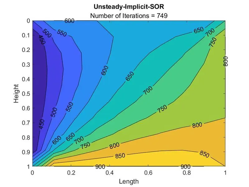

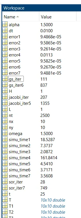
Workspace Screenshot after successful run of the code:

Conclusions:

1) From the output figures and workspace data it is clear that among the three iterative methods the SOR converges faster than the Gauss Seidel and Jacobi method. Jacobi is slower than the Gauss Seidel method.

2) From the iteration counters and simulation time it is clear that the steady state sovers converge faster than the unsteady state solvers.

3) Among the unsteady state solvers the implicit solvers have the faster rate of convergence than the explicit solver.

4)The error and simulation time values from workspace, implies that the Unsteady Explicit solver requires a higher number of iterations to attain the steady state solution.

5) Simulation times obtained here are on a higher side due to the fact that the contour plot is plotted inside the loop and results of each iteration are paused for 0.01 sec.