Week 7 - Simulation of a 1D Super-sonic nozzle flow simulation using Macormack Method
Aim: Simulation of 1D supersonic nozzle flow using MacCormack Method
Theory:
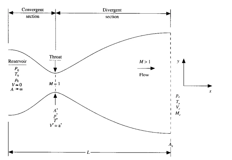
Schematic for subsonic supersonic isentropic flow through convergent divergent nozzle:
Control Volume for deriving the partial differential equations for unsteady quasi 1D flow:
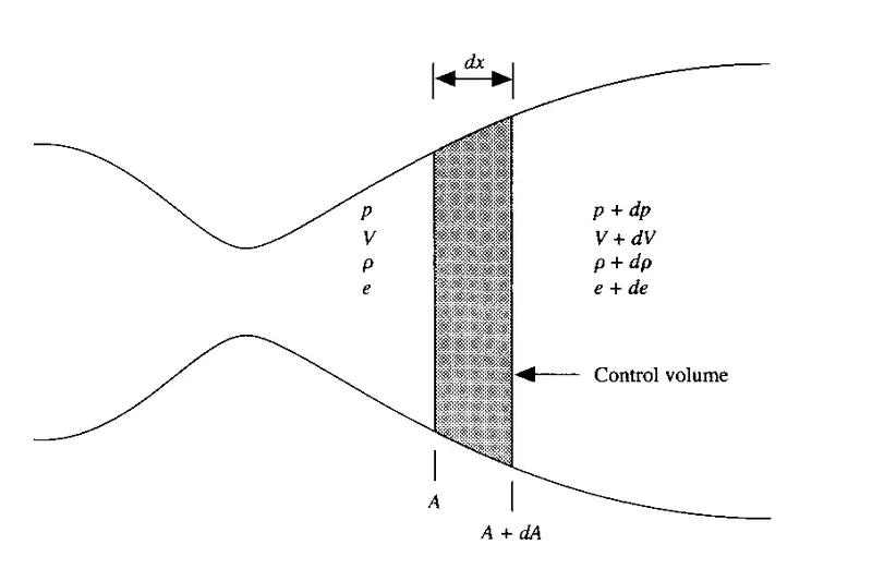
Using integral forms of continuity, momentum and energy equations the Nonconservative forms of continuity, momentum and energy equations appropriate for unsteady quasi 1D flow are depicted as follows:
Nonconservative form of equations are arranged using `e=C_v T` , `p=rhoRT` & `(delp)/(delx) = R (rho(delT)/(delx) + T(delrho)/(delx))` .
Continuity equation: `(del(rhoA))/(delt) + rhoA (delV)/(delx) + rhoV(delA)/(delx) +VA(delrho)/(delx) =0`
x-momentum equation: `rho (delV)/(delt) + rhoV (delV)/(delx) =-R (rho(delT)/(delx) + T(delrho)/(delx)) `
Energy Equation: `rhoC_v (delT)/(delt) + rhoVC_v (delT)/(delx) = -rhoRT ((delV)/(delx) + V(del(lnA))/(delx))`
Similarly the Conservative form of the continuity, momentum and energy equations appropriate for unsteady quasi 1D flow are as follows:
Continuity equation: `(del(rhoA))/(delt)+(del(rhoAV))/(delx) =0`
x-momentum equation: `(del(rhoAV))/(delt)+(del(rhoAV^2+pA))/(delx) =p(delA)/(delx)`
Energy Equation: `(del(rhoA(e+V^2/2)))/(delt)+(del(rhoA(e+V^2/2)V+pAV))/(delx) =0`
Above equations are in the dimensional form which are then converted into nondimensional form by making the parameters nondimensional (Normalised form of parameter), are as follows:
Normalised form of Parameters:
`"Temperature (T)" ` and `"Density (rho)" ` are normalised with the help of temperature and density at reservoir hence ` T'=T/T_0` and `rho'=rho/rho_0` ;
Distance along x axis is normalised using the total length (L) of nozzle i.e. `x'=x/L ` ;
Velocity is normalised with the help of speed of sound at the reservoir,
speed of sound at reservoir is `a_0= sqrt( gammaRT_0)` hence `V'=V/a_0` ;
Time is normalised as the `t'= t/(L/a_0)` ;
Area is normalised using sonic throat area as `A'=A/A^**` .
Pressure is normalised with reservoir pressure `p'=p/p_0`
i .e. ` p'= (rhoRT)/(rho_0RT_0) =rho'T'` ;
Internal Energy is normalised as `e'=e/e_0` where
`e_0=C_vT_0=R/(gamma-1) T_0` ;
Thus the Nondimensional form of Nonconservative Equations are follows:
Nondimensional Continuity equation (Nonconservative Form):
`(delrho')/(delt') =- rho' (delV')/(delx') - rho'V'(del(lnA'))/(delx') - V'(delrho')/(delx')`
Nondimensional x-momentum equation (Nonconservative Form):
`(delV')/(delt') = - V' (delV')/(delx') -1/gamma ((delT')/(delx') + (T')/(rho') (delrho')/(delx')) `
Nondimensional Energy Equation (Nonconservative Form):
`(delT')/(delt') = -V'(delT')/(delx') - (gamma-1)T' ((delV')/(delx') + V'(del(lnA'))/(delx'))`
Similarly the Nondimensional form of the Conservative Equations are as follows:
Nondimensional Continuity equation (Conservative Form):
`(del(rho'A'))/(delt')+(del(rho'A'V'))/(delx') =0`
Nondimensional x-momentum equation (Conservative Form):
`(del(rho'A'V'))/(delt')+(del(rho'A'V'^2 + 1/gamma p'A'))/(delx') = 1/gamma p'(delA')/(delx')`
Nondimensional Energy Equation (Conservative Form):
`(del(rho'A'((e')/(gamma-1) + 1/gamma V'^2/2)))/(delt')+(del(rho'A'((e')/(gamma-1) + gamma/2 V'^2)V'+p'A'V'))/(delx') =0`
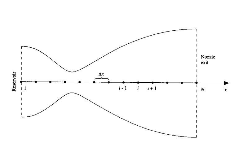
Grid Point distribution along the nozzle :
Methodology:
I) MacCormack's Technique for Nonconservative approach :
MacCormack's Technique is the predictor-corrector method , in the predictor step where the time derivatives of the flow field variables are predicted using a forward difference scheme for spatial derivatives. Using these predicted time derivatives the predicted values of flow field variables are calculated as the sum of initial values of flow field variables and the product of predicted time derivatives with timestep value used for calculation. Then these predicted values are used for corrector steps.
In the corrector step the corrected time derivatives of the flow field variables are obtained using backward difference scheme for the spatial derivatives, by using the predicted values for flow field variables (as obtained in the the predictor step).
Then the average time derivatives of flow field variables are obtained as the average of the predictor step time derivative and corrector step time derivative values.
Then the updated flow field variable values for next time step as the sum of initial values of flow field variables and the product of average time derivatives with timestep value used for calculation.
above calculations are repeated for the required number of iterations till the steady state solution is obtained.
Time Step calculation: As MacCormack's technique is an explicit method it has satisfy the CFL criteria for the solution to be stable, for that the time step value at each node is calculated as
`Deltat_i = C*Deltax/(a_i + V_i)` , which is same as `Deltat'_i = C*(Deltax')/(a'_i + V'_i)`
For any assumed value of C (less than equal to 1) the calculated time step values at each node for same time step are different as speed of sound and velocity of flow is different at each node thus minimum of time step values calculated all nodes is used as the time step value for calculations at each time iteration
i.e. `Deltat^t = min {Deltat_1^t,Deltat_2^t,Deltat_3^t,........,Deltat_n^t} `
where the value of normalised speed of sound (a') is calculated as follows
i.e. `a'= a/a_o=sqrt((gammaRT)/(gammaRT_o))= sqrt(T')` .
Boundary Conditions for subsonic inflow and supersonic outflow as follows
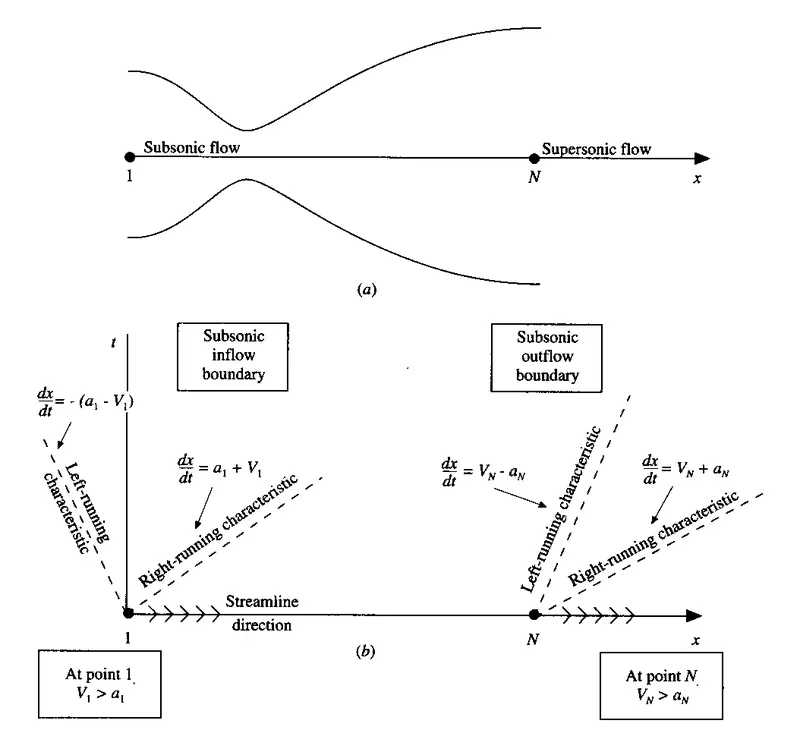
Subsonic inflow boundary conditions (at node 1)
`V'_1 = 2*V'_2 - V'_3 ` - floating parameter
`rho'_1 = 1` - fixed parameters (independent of time)
`T'_1 = 1` - fixed parameters (independent of time)
Supersonic outflow boundary conditions (at node n)
`V'_n = 2*V'_(n-1) - V'_(n-2) ` - floating parameter
`rho'_n = 2*rho'_(n-1) - rho'_(n-2) ` - floating parameter
`T'_n = 2*T'_(n-1) - T'_(n-2) ` - floating parameter
Nozzle Shape and Initial Conditions (at t=0)
For `0 <= x' <=3`
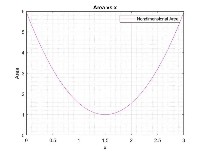
Nozzle shape: `A'(x') = 1+ 2.2(x'-1.5)^2`
Initial conditions:
`rho'(x') = 1 - 0.3146x'` - initial condition for `rho'` ,
`T'(x') = 1 - 0.2314x'` - initial condition for `T'`,
`V'(x') = (0.1 + 1.09x')T'^0.5` - initial condition for `V'` .
II) MacCormack's Technique for Conservative approach :
From the Nondimensional form of the conservative equations, Let us define the terms of solution vector U , elements of Flux vector F and elements of Source term J as follows:
`U_1 = rho'A'`
`U_2 = rho'A'V'`
`U_3 = rho'A'((e')/(gamma-1) + gamma/2 V'^2)`
`F_1 = rho'A'V'`
`F_2 = rho'A'V'^2 + 1/gamma p'A'`
`F_3 = rho'A'V' ((e')/(gamma-1) + gamma/2 V'^2) +p'A'V' `
`J_2 = 1/gamma p'(delA')/(delx')`
with these elements Nondimensional form of the conservative equations become
`(delU_1)/(delt') = -(delF_1)/(delx') `
`(delU_2)/(delt') = -(delF_2)/(delx') + J_2`
`(delU_3)/(delt') = -(delF_3)/(delx')`
To use MacCormack's Technique for conservative approach, in the predictor step where the time derivatives of the solution vector field variables are predicted using a forward difference scheme for flux vector spatial derivatives. Using these predicted time derivatives the predicted values of solution vector field variables are calculated as the sum of initial values of solution vector field variables and the product of predicted time derivatives of solution vector field with timestep value used for calculation. Then these predicted values are used for corrector steps.
In the corrector step the corrected time derivatives of the solution vector field variables are calculated using backward difference scheme for the flux vector spatial derivatives and source term spatial derivatives, by using the primitive variable's values for evaluation of terms of solution vector ,flux vector and source (i.e. primitive variables obtained from the solution vector obtained in the the predictor step). The Pure form of the flux vector and source term as used for this purpose.
The Pure form of the Flux terms and Source term are as follows:
`F_1 = U_2`
`F_2 = U_2^2/U_1 + (gamma-1)/gamma (U_3 - gamma/2 U_2^2/U_1)`
`F_3 = gamma (U_2 U_3)/U_1 + gamma(gamma-1)/2 (U_3^2 /U_1^2)`
`J_2= (gamma-1)/gamma (U_3 - gamma/2 U_2^2/U_1) (del(lnA'))/(delx')`
Then the average time derivatives of solution vector terms are obtained as the average of the predictor step time derivative and corrector step time derivative values for corresponding term.
Then the solution vector terms are updated for next time step as the sum of initial values of solution vector terms and the product of average time derivatives with timestep value used for calculation.
The primitive variable are evaluated from the solution vector terms as follows:
`rho'= U_1/A'`
`V' = U_2/U_1`
`T'=e'=(gamma-1) (U_3/U_1 - gamma/2 V'^2)`
`p'=rho'T'`
above steps are repeated for the required number of iterations till the steady state solution is obtained.
Time Step calculation: It is same as mentioned in the nonconservative approach.
Boundary Conditions for subsonic inflow and supersonic outflow as follows
Subsonic inflow boundary conditions (at node 1)
`(U_1)_1 = (rho'A')_1 ` - fixed parameter
`(U_2)_1 = 2*(U_2)_(n-1) - (U_2)_(n-2)` - floating parameter
`(U_3)_1=(U_1)_1 ((T')/(gamma-1) + gamma/2 V'^2)` - floating parameter
Supersonic outflow boundary conditions (at node n)
`(U_1)_n = 2*(U_1)_(n-1) - (U_1)_(n-2) ` - floating parameter
`(U_2)_n = 2*(U_2)_(n-1) - (U_2)_(n-2) ` - floating parameter
`(U_3)_n = 2*(U_3)_(n-1) - (U_3)_(n-2) ` - floating parameter
Nozzle Shape and Initial Conditions (at t=0)
Nozzle shape: `A'(x') = 1+ 2.2(x'-1.5)^2` for `0 <= x' <=3`
Initial conditions:
`rho'(x') = 1 ` - initial condition for `rho'` for `0 <= x' <=0.5` ,
`T'(x') = 1 ` - initial condition for `T'` for `0 <= x' <=0.5`,
`rho'(x') = 1 - 0.366(x'-0.5)` - initial condition for `rho'` for `0.5 <= x'<=1.5` ,
`T'(x') = 1 - 0.167(x'-0.5)` - initial condition for `T'` for `0.5 <= x'<=1.5`,
`rho'(x') = 0.634 - 0.3879(x'-1.5)` - initial condition for `rho'` for `1.5 <= x'<=3` ,
`T'(x') = 0.833 - 0.3507(x'-1.5)` - initial condition for `T'` for `1.5 <= x'<=3`,
`U_2 = 0.59 ` hence `V'=0.59/(rho'A')`
hence initial values of `U_1` ,`U_2` and `U_3` are given as
`U_1 =rho'A'`
`U_2 = rho'A'V'`
`U_3 = rho'A'((T')/(gamma-1) + gamma/2 V'^2)` .
The required results are plotted for both nonconservative and conservative approach and cross check with the exact analytical solution available for the problem.
Main Code:
close all
clear all
clc

%inputs
n=[31,61,91];              % No of nodes
L=3;                       % Length of domain
gamma=1.4;                 %Adiabatic const for air

% time steps
nt=1400;
C=0.5;             %CFL No

for i=1:length(n)

    x=linspace(0,L,n(i)); % x coordinate of nodes
    dx=3/(n(i)-1);        % increment of x

% Function call for Nonconservative approach
[x_nc,a_nc,rho_nc,v_nc,t_nc,M_nc,p_nc,mdot_nc,A_nc,A1_nc]=MacCormack_nonconservative(n(i),x,dx,nt,C);
   rhonc(i)= rho_nc((n(i)+1)/2);  % Nondimensional density at throat for varoius nodes
   tnc(i)= t_nc((n(i)+1)/2);      % Nondimensional temperature at throat for varoius nodes
   pnc(i)= p_nc((n(i)+1)/2);      % Nondimensional pressure at throat for varoius nodes
   Mnc(i)= M_nc((n(i)+1)/2);      % Mach Number at throat for varoius nodes

% Function call for Conservative approach
[x_con,a_con,rho_con,v_con,t_con,M_con,p_con,mdot_con,A_con,A1_con]=MacCormack_conservative(n(i),x,dx,nt,C);
   rhocon(i)= rho_con((n(i)+1)/2); % Nondimensional density at throat for varoius nodes
   tcon(i)= t_con((n(i)+1)/2);     % Nondimensional temperature at throat for varoius nodes
   pcon(i)= p_con((n(i)+1)/2);     % Nondimensional pressure at throat for varoius nodes
   Mcon(i)= M_con((n(i)+1)/2);     % Mach Number at throat for varoius nodes

if n(i)==31
%Comparision of nondimensional massflowrate inside the nozzle between nonconservative and conservative approach
  figure(6)
     plot(x,mdot_nc,'DisplayName','Nondimensional massflowrate_nc')
     hold on
     plot(x,mdot_con,'DisplayName','Nondimensional massflowrate_con')
     title({'Nonconservative & Conservative:Nondimensional massflow rate inside the nozzle'})
     xlabel('x')
     ylabel('Nondimensional massflowrate')
     legend ('Nondimensional massflowrate-Nc','Nondimensional massflowrate-Con',Location='best')
     grid on
     grid minor
     saveas(gcf,'Comparision of nondimensional massflowrate inside nozzle for NC & Con','jpg')
end
end
%% Grid Independence study table
Perticulars= {'Exact Solution';'Nonconservative form(n=31)';'Nonconservative form(n=61)';'Nonconservative form(n=91)';'Conservative form(n=31)';'Conservative form(n=61)';'Conservative form(n=91)'};
Nondimensional_Rho = [0.634;rhonc(1,1);rhonc(1,2);rhonc(1,3);rhocon(1,1);rhocon(1,2);rhocon(1,3)];
Nondimensional_Temp = [0.833;tnc(1,1);tnc(1,2);tnc(1,3);tcon(1,1);tcon(1,2);tcon(1,3)];
Nondimensional_Press = [0.528;pnc(1,1);pnc(1,2);pnc(1,3);pcon(1,1);pcon(1,2);pcon(1,3)];
Mach_Number = [1;Mnc(1,1);Mnc(1,2);Mnc(1,3);Mcon(1,1);Mcon(1,2);Mcon(1,3)];
T=table(Perticulars,Nondimensional_Rho,Nondimensional_Temp,Nondimensional_Press,Mach_Number);

%% Parameter variation with varying no of nodes
     figure(7)
     plot(n,rhonc,'ro-',n,tnc,'bo-',n,pnc,'go-',n,Mnc,'mo-')
     hold on
     plot(n,rhocon,'r*--',n,tcon,'b*--',n,pcon,'g*--',n,Mcon,'m*--')
     title({'Comparision of primitive variable values for varying nodes'})
     xlabel('No of nodes')
     ylabel('Rho,Temp,Pressure & Mach Number')
     legend ('rhonc','tnc','pnc','Mnc','rhocon','tcon','pcon','Mcon',Location='southeastoutside')
     grid on
     grid minor
     saveas(gcf,'Comparision of primitive variable values for varying nodes','jpg')
Function code for Nonconservative approach:
function [x,a,rho,v,t,M,p,mdot,A,A1]=MacCormack_nonconservative(n,x,dx,nt,C)

%calculating initial profiles
rho= 1- 0.3146*x;           % nondimentional density
t = 1-0.2314*x;             % nondimentional temperature (=t)
v= (0.1 + 1.09*x).*t.^0.5;  % nondimentional velocity
a= 1+(2.2*(x-1.5).^2);      % area profile as function of x
M= v./(t.^0.5);             % Mach Number
p= rho.*t;                  % nondimentional pressure
mdot=rho.*a.*t;             % nondimentional mass flow rate
gamma=1.4;                  % Adiabatic const for air

% time steps
%nt=1400;
%dt=0.01;
%C=0.5;

A=[x' a' rho' v' t' p' M' mdot']; %Intial conditions

% Area profile plot
if n==31
    figure(11)
     plot(x,a,'color','m','DisplayName','Nondimensional Area Profile')
     title('Area vs x')
     xlabel('x')
     ylabel('Area')
     axis([0 3 0 6])
     legend ('Nondimensional Area')
     grid on
     grid minor
end

%outer time loop
for k=1:nt

    rho_old=rho;
    v_old=v;
    t_old=t;


    %time step calculation
    dtm=zeros(1,n);
    for j=1:n
     dtm(j)=C*dx/(sqrt(t(j))+v(j));
    end
     dt=min(dtm);

   %predictor step
    for j=2:n-1
        dvdx=(v(j+1)-v(j))/dx;
        drhodx=(rho(j+1)-rho(j))/dx;
        dtdx= (t(j+1)-t(j))/dx;
        dlogadx=(log(a(j+1))-log(a(j)))/dx;

        % continuity equation
        drhodt_p(j)=-rho(j)*dvdx-rho(j)*v(j)*dlogadx-v(j)*drhodx ;

        % momentum equation
        dvdt_p(j)=-v(j)*dvdx -(1/gamma)*(dtdx+((t(j)/rho(j))*drhodx));

        % Energy equation
        dtdt_p(j)=-v(j)*dtdx-((gamma-1)*t(j)*(dvdx +(v(j)*dlogadx)));

        %solution update
        rho(j)=rho(j) + drhodt_p(j)*dt;
        v(j)= v(j) + dvdt_p(j)*dt;
        t(j)= t(j) + dtdt_p(j)*dt;

    end

    %corrector step
    for j=2:n-1
        dvdx=(v(j)-v(j-1))/dx;
        drhodx=(rho(j)-rho(j-1))/dx;
        dtdx= (t(j)-t(j-1))/dx;
        dlogadx=(log(a(j))-log(a(j-1)))/dx;

        % continuity equation
        drhodt_c(j)=-rho(j)*dvdx-rho(j)*v(j)*dlogadx-v(j)*drhodx ;

        % momentum equation
        dvdt_c(j)=-v(j)*dvdx -(1/gamma)*(dtdx+((t(j)/rho(j))*drhodx));

        % Energy equation
        dtdt_c(j)=-v(j)*dtdx-((gamma-1)*t(j)*(dvdx +(v(j)*dlogadx)));

    end
        %compute the average time derivative
        drhodt=0.5*(drhodt_p + drhodt_c);
        dvdt=0.5*(dvdt_p + dvdt_c);
        dtdt=0.5*(dtdt_p + dtdt_c) ;

    %solution update
     for i=2:n-1

          rho(i)=rho_old(i) + drhodt(i)*dt;
          v(i)= v_old(i) + dvdt(i)*dt;
          t(i)= t_old(i) + dtdt(i)*dt;
          M(i)=v(i)/(t(i)^0.5);
          p(i)=rho(i)*t(i);
          mdot(i)=rho(i)*a(i)*v(i);
     end

     % Apply the boundary conditions
     % inlet
     v(1)=2*v(2)-v(3);
     M(1)=v(1)/(t(1)^0.5);
     p(1)=rho(1)*t(1);
     mdot(1)=rho(1)*a(1)*v(1);

     % outlet
     v(n)=2*v(n-1)-v(n-2);
     rho(n)=2*rho(n-1)-rho(n-2);
     t(n)=2*t(n-1)-t(n-2);
     M(n)=v(n)/(t(n)^0.5);
     p(n)=rho(n)*t(n);
     mdot(n)=rho(n)*a(n)*v(n);

     %drhodt_16(k)=abs(drhodt(16));
     %dvdt_16(k)=abs(dvdt(16));
     %dtdt_16(k)=abs(dtdt(16));

     % Recording time wise variation of required variables
         rho_g((1:n),k)= rho(1:n);      % nondimensional density
         t_g((1:n),k)= t(1:n);          % nondimensional tempearture
         v_g((1:n),k)= v(1:n);          % nondimensional velocity
         p_g((1:n),k)= p(1:n);          % nondimensional pressure
         M_g((1:n),k)= M(1:n);          % Mach number
         mdot_16(k)=rho(16)*a(16)*v(16);% nondimensional Mass flow rate at throat
         mdot1((1:n),k)=mdot(1:n);       % non dimensiona Mass flow rate as calculated


     if k==1
         A1=[x' a' rho' v' t' p' M' mdot'];
     end

end

B=[x' a' rho' v' t' p' M' mdot'];

if n==31
%figure(11)
     saveas(figure(11),'Nondimensional Area Profile-NC','jpg')

%% Variation of primitive variables inside the nozzle
     figure(12)
     plot(x,v,'color','r','DisplayName','Velocity')
     hold on
     plot(x,rho,'color','b','DisplayName','Density')
     hold on
     plot(x,t,'color','g','DisplayName','Temperature')
     hold on
     plot(x,p,'color','c','DisplayName','Pressure')
     hold on
     plot(x,M,'color','m','DisplayName','Mach Number')
     hold on
     text1=sprintf('Number of iteration =%d',k);
     title({text1;'Vel,rho,t,p,M vs x'})
     xlabel('x')
     ylabel('Vel,Rho,t,p,M')
     legend ('Velocity','Density','Temperature','Pressure','Mach Number',Location='northwest')
     grid on
     grid minor
     saveas(gcf,'Steady state distribution of primitive variables inside the nozzle-NC','jpg')

%% Time wise variation of primitive variables at throat
     figure(13)
     plot((1:nt),rho_g(16,:),'color','b','DisplayName','Nondimensional density at throat')
     hold on
     plot((1:nt),t_g(16,:),'color','r','DisplayName','Nondimensional temperature at throat')
     hold on
     plot((1:nt),v_g(16,:),'color','g','DisplayName','Nondimensional velocity at throat')
     hold on
     title({'Parameters at throat vs No of iterations'})
     xlabel('No of Iterations')
     ylabel('rho,v,t')
     legend(Location='northeast')
     grid on
     grid minor
     saveas(gcf,'Time wise variation of primitive variables at throat-NC','jpg')

 %%   plotting of mass flowrate after every 100 iterations
     l=(1:100:nt);
     for q=1:length(l)
         mdot2((1:n),q)=mdot1((1:n),l(q));
         figure(14)
         plot((1:n),mdot2((1:n),q),'DisplayName',num2str(l(q)))
         hold on
         xlabel('x')
         ylabel('Normalised mass flowrate')
         title('Nondimensional massflow rate inside nozzle at varoius time steps')
         legend(Location="eastoutside")
         grid on
     end
     saveas(gcf,'Nondimensional massflowrate insde the nozzle at various timestep-NC','jpg')
  %% plotting normalised massflowrate,pressure and Mach number at throat Vs time steps
     figure(15)
     plot((1:nt),mdot1(16,:),'color','c')
     hold on
     plot((1:nt),p_g(16,:),'color','m')
     hold on
     plot((1:nt),M_g(16,:),'color','k')
     hold on
     xlabel('Number of iterations')
     ylabel('mdot,p,M')
     title({'Parameters at throat vs No of iterations'})
     legend('normalised massflowrate at throat','normalised pressure at throat','Mach number at throat')
     grid on
     grid minor
     saveas(gcf,'Time wise variation of Nondimensional massflowrate,p & M at throat-NC','jpg')
end
end
Function code for Conservative approach:
function [x,a,rho,v,t,M,p,mdot,A,A1]=MacCormack_conservative(n,x,dx,nt,C)

%inputs
%n=31;              % No of nodes
%L=3;               % Length of domain
%x=linspace(0,L,n); % x coordinate of nodes
%dx=3/(n-1);        % increment of x
gamma=1.4;          %Adiabatic const for air

% time steps
%nt=1400;
%C=0.5;

%calculating initial profiles of normalised rho & t
for k=1:n
    if (0<=x(k))&&(x(k)<=0.5)
        rho(k)= 1;
        t(k)=1;
    elseif (0.5<= x(k))&&(x(k)<=1.5)
        rho(k)= 1- 0.366*(x(k)-0.5);
        t(k)= 1- 0.167*(x(k)-0.5);
    elseif (1.5<=x(k)) && (x(k)<=3)
        rho(k)= 0.634 - 0.3879*(x(k)-1.5);
        t(k)= 0.833 - 0.3507*(x(k)-1.5);
    end
      a(k)= 1+2.2*(x(k)-1.5).^2;      % normalised area profile
      v(k)= 0.59/(rho(k)*a(k));       % Normalised initial velocity based on mass flow rate

      % Initialisation of solution vector terms U1,U2 & U3
        U1(k)=rho(k)*a(k);
        U2(k)=U1(k)*v(k);
        U3(k)=U1(k)*((t(k)/(gamma-1))+((gamma/2)*v(k)^2));

end

A=[x' a' rho' v' t' U2' U1' U2' U3']; %Initial Condition

%Area profile plot
   if n==31
     figure(1)
     plot(x,a,'color','m','DisplayName','Nondimensional Area Profile')
     title('Area vs x')
     xlabel('x')
     ylabel('Area')
     axis([0 3 0 6])
     legend ('Nondimensional Area')
     grid on
     grid minor
   end

dtm=zeros(1,n);
F1=zeros(1,n);
F2=zeros(1,n);
F3=zeros(1,n);
J2=zeros(1,n);

%outer time loop
for k=1:nt

    rho_old=rho;
    v_old=v;
    t_old=t;
    P(:,(1:n),k)=[rho_old(1:n);v_old(1:n);t_old(1:n)];
    U1_old=U1;
    U2_old=U2;
    U3_old=U3;
    U(:,(1:n),k)=[U1(1:n);U2(1:n);U3(1:n)];

    % Flux Vector and min time step calculation
    for j=1:n
        F1(j)= U2(j);
        F2(j)=((U2(j)^2/U1(j))+(((gamma-1)/gamma)*(U3(j)-((gamma/2)*(U2(j)^2/U1(j))))));
        F3(j)=((gamma*U2(j)*U3(j)/U1(j))-((gamma*(gamma-1)/2)*(U2(j)^3/U1(j)^2)));
        F_p(:,j,k)=[F1(j);F2(j);F3(j)];
        dtm(j)= (C*dx)/(sqrt(t(j))+v(j));
        Dtm(j,k)=dtm(j);
    end

   % min time step calculation
       dt(k)=min(dtm(1:n));
       %dt(k)=0.0267;

   % predictor step
    for j=2:n-1
        dF1dx=(F1(j+1)-F1(j))/dx;
        dF2dx=(F2(j+1)-F2(j))/dx;
        dF3dx=(F3(j+1)-F3(j))/dx;
        J2(j)=((1/gamma)*rho(j)*t(j)*(a(j+1)-a(j))/dx); %Source term calculation
        %J2_p(:,j,k)=J2(j);
        %dlogadx=(log(a(j+1))-log(a(j)))/dx;
        %J2(j)=(((gamma-1)/gamma)*(U3(j)-((gamma/2)*(U2(j)^2/U1(j)))))*dlogadx; %Source term calculation

        % continuity equation
           dU1dt_p(j)= -dF1dx;
        % momentum equation
           dU2dt_p(j)= -dF2dx + J2(j);
        % Energy equation
           dU3dt_p(j)= -dF3dx;
        % solution update
           U1(j)= U1(j) + dU1dt_p(j)*dt(k);
           U2(j)= U2(j) + dU2dt_p(j)*dt(k);
           U3(j)= U3(j) + dU3dt_p(j)*dt(k);
           %U_p(:,j,k)=[U1(j);U2(j);U3(j)];

       % updating rho v t and Flux vector terms
           rho(j)= U1(j)/a(j);
           v(j)= U2(j)/ U1(j);
           t(j)=(gamma-1)*((U3(j)/U1(j))-((gamma/2)*v(j)^2));
           F1(j)= U2(j);
           F2(j)=((U2(j)^2/U1(j))+(((gamma-1)/gamma)*(U3(j)-((gamma/2)*(U2(j)^2/U1(j))))));
           F3(j)=((gamma*U2(j)*U3(j)/U1(j))-((gamma*(gamma-1)/2)*((U2(j)^3/U1(j)^2))));
           %F_c(:,j,k)=[F1(j);F2(j);F3(j)];

    end

    % Updating Inflow floating boundary conditions
         U1(1)=rho(1)*a(1);
         U2(1)=2*U2(2)-U2(3);
         U3(1)=U1(1)*((t(1)/(gamma-1))+((gamma/2)*(U2(1)/U1(1))^2));
         rho(1)= U1(1)/a(1);
         v(1)= U2(1)/ U1(1);
         t(1)=(gamma-1)*((U3(1)/U1(1))-((gamma/2)*v(1)^2));
         p(1)=rho(1)*t(1);
         M(1)=v(1)/sqrt(t(1));
         F1(1)= U2(1);
         F2(1)=((U2(1)^2/U1(1))+(((gamma-1)/gamma)*(U3(1)-((gamma/2)*(U2(1)^2/U1(1))))));
         F3(1)=((gamma*U2(1)*U3(1)/U1(1))-((gamma*(gamma-1)/2)*((U2(1)^3/U1(1)^2))));

    %corrector step
    for j=2:n-1
        dF1dx=(F1(j)-F1(j-1))/dx;
        dF2dx=(F2(j)-F2(j-1))/dx;
        dF3dx=(F3(j)-F3(j-1))/dx;
        J2(j)=((1/gamma)*rho(j)*t(j)*(a(j)-a(j-1))/dx); %source term calculation
        %dlogadx=(log(a(j))-log(a(j-1)))/dx;
        %J2(j)=(((gamma-1)/gamma)*(U3(j)-((gamma/2)*(U2(j)^2/U1(j)))))*dlogadx;
        %J2_c(:,j,k)=J2(j);

        % continuity equation
          dU1dt_c(j)= -dF1dx;
        % momentum equation
          dU2dt_c(j)= -dF2dx + J2(j);
        % Energy equation
          dU3dt_c(j)= -dF3dx;

    end

     %compute the average time derivatives of solution vector terms
        dU1dt=0.5*(dU1dt_p + dU1dt_c);
        dU2dt=0.5*(dU2dt_p + dU2dt_c);
        dU3dt=0.5*(dU3dt_p + dU3dt_c);

     for i=2:n-1
          %solution update for next time step
          U1(i)= U1_old(i) + dU1dt(i)*dt(k);
          U2(i)= U2_old(i) + dU2dt(i)*dt(k);
          U3(i)= U3_old(i) + dU3dt(i)*dt(k);
          rho(i)= U1(i)/a(i);
          v(i)= U2(i)/ U1(i);
          t(i)=(gamma-1)*((U3(i)/U1(i))-((gamma/2)*v(i)^2));
          p(i)=rho(i)*t(i);
          M(i)=v(i)/sqrt(t(i));
          mdot(i)=rho(i)*a(i)*v(i);
          F1(i)= U2(i);
          F2(i)=((U2(i)^2/U1(i))+(((gamma-1)/gamma)*(U3(i)-((gamma/2)*(U2(i)^2/U1(i))))));
          F3(i)=((gamma*U2(i)*U3(i)/U1(i))-((gamma*(gamma-1)/2)*((U2(i)^3/U1(i)^2))));
     end

     % Update and apply the boundary conditions
     % inlet
         U1(1)=rho(1)*a(1);
         U2(1)=2*U2(2)-U2(3);
         U3(1)=U1(1)*((t(1)/(gamma-1))+((gamma/2)*(U2(1)/U1(1))^2));
         rho(1)= U1(1)/a(1);
         v(1)= U2(1)/ U1(1);
         t(1)=(gamma-1)*((U3(1)/U1(1))-((gamma/2)*v(1)^2));
         p(1)=rho(1)*t(1);
         M(1)=v(1)/sqrt(t(1));
         mdot(1)=rho(1)*a(1)*v(1);
         F1(1)= U2(1);
         F2(1)=((U2(1)^2/U1(1))+(((gamma-1)/gamma)*(U3(1)-((gamma/2)*(U2(1)^2/U1(1))))));
         F3(1)=((gamma*U2(1)*U3(1)/U1(1))-((gamma*(gamma-1)/2)*((U2(1)^3/U1(1)^2))));

     % outlet
         U1(n)=2*U1(n-1)-U1(n-2);
         U2(n)=2*U2(n-1)-U2(n-2);
         U3(n)=2*U3(n-1)-U3(n-2);
         rho(n)= U1(n)/a(n);
         v(n)= U2(n)/ U1(n);
         t(n)=(gamma-1)*((U3(n)/U1(n))-((gamma/2)*v(n)^2));
         p(n)=rho(n)*t(n);
         M(n)=v(n)/sqrt(t(n));
         mdot(n)=rho(n)*a(n)*v(n);
         F1(n)= U2(n);
         F2(n)=((U2(n)^2/U1(n))+(((gamma-1)/gamma)*(U3(n)-((gamma/2)*(U2(n)^2/U1(n))))));
         F3(n)=((gamma*U2(n)*U3(n)/U1(n))-((gamma*(gamma-1)/2)*((U2(n)^3/U1(n)^2))));

       % Recording time wise variation of required variables
         rho_g((1:n),k)= rho(1:n);      % nondimensional density
         t_g((1:n),k)= t(1:n);          % nondimensional tempearture
         v_g((1:n),k)= v(1:n);          % nondimensional velocity
         p_g((1:n),k)= p(1:n);          % nondimensional pressure
         M_g((1:n),k)= M(1:n);          % Mach number
         U2_g((1:n),k)= U2(1:n);        % nondimensional Mass flow rate as U2
         mdot_16(k)=rho(16)*a(16)*v(16);% nondimensional Mass flow rate at throat
         mdot1(k,(1:n))=rho.*a.*v;       % non dimensiona Mass flow rate as calculated

     if k==1
         A1=[x' a' rho' v' t' p' M' mdot1(1,:)' U1' U2' U3'];
     end

end

B=[x' a' rho' v' t' p' M' mdot1(end,:)' U1' U2' U3'];

if n==31
%figure(1)
     saveas(figure(1),'NonDimensional Area Profile-Con','jpg')

%% Variation of primitive variables inside the nozzle
     figure(2)
     plot(x,v,'color','r','DisplayName','Velocity')
     hold on
     plot(x,rho,'color','b','DisplayName','Density')
     hold on
     plot(x,t,'color','g','DisplayName','Temperature')
     hold on
     plot(x,p,'color','c','DisplayName','Pressure')
     hold on
     plot(x,M,'color','m','DisplayName','Mach Number')
     hold on
     text1=sprintf('Number of iteration =%d',k);
     title({text1;'Vel,rho,t,p,M vs x'})
     xlabel('x')
     ylabel('Vel,Rho,t,p,M')
     legend ('Velocity','Density','Temperature','Pressure','Mach Number',Location='northwest')
     grid on
     grid minor
     saveas(gcf,'Steady state distribution of primitive variables inside the nozzle-Con','jpg')

%% Time wise variation of primitive variables at throat
     figure(3)
     plot((1:nt),rho_g(16,:),'color','b','DisplayName','Nondimensional density at throat')
     hold on
     plot((1:nt),t_g(16,:),'color','r','DisplayName','Nondimensional temperature at throat')
     hold on
     plot((1:nt),v_g(16,:),'color','g','DisplayName','Nondimensional velocity at throat')
     hold on
     title({'Parameters at throat vs No of iterations'})
     xlabel('No of Iterations')
     ylabel('rho,v,t')
     legend(Location='east')
     grid on
     grid minor
     saveas(gcf,'Time wise variation of primitive variables at throat-Con','jpg')

 %%   plotting of mass flowrate after every 100 iterations
     l=(1:100:nt);
     for q=1:length(l)
         mdot2(q,(1:n))=mdot1(l(q),(1:n));
         figure(4)
         plot((1:n),mdot2(q,(1:n)),'DisplayName',num2str(l(q)))
         hold on
         xlabel('x')
         ylabel('normalised mass flowrate')
         title('Nondimensional massflow rate inside nozzle at varoius time steps')
         legend(Location="eastoutside")
         grid on
     end
    saveas(gcf,'Nondimensional massflowrate inside the nozzle at various timestep-Con','jpg')
%% Time wise variation of nondimensional massflowrate at throat
     figure(5)
     plot((1:nt),mdot_16,'DisplayName','Nondimensional massflowrate at throat')
     hold on
     plot((1:nt),p_g(16,:),'color','m','DisplayName','Nondimensional pressure at throat')
     hold on
     plot((1:nt),M_g(16,:),'color','k','DisplayName','Mach Number at throat')
     title({'Parameters at throat vs No of iterations'})
     xlabel('No of iterations')
     ylabel('Nondimensional massflowrate at throat')
     legend (Location='northeast')
     grid on
     grid minor
     saveas(gcf,'Time wise variation of nondimensional massflowrate at throat-Con','jpg')

end
end
Initial boundary conditions , Variable after 1st time step and Final steady state solution for nonconservative as well as conservative approach are compared with references given in the chapter 7 of the book " Computational Fluid Dynamics" by John D. Anderson, found in close match with acceptable tolerance.
The require results are plotted as follows:
1) Nondimensional Area profile -Nonconservative approach
2) Nondimensional Area profile -Conservative approach
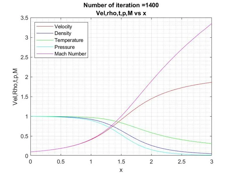
3) Variation of primitive variables inside nozzle - Nonconservative approach
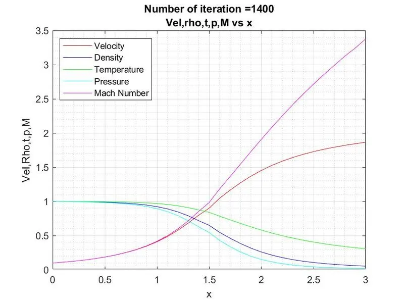
4)Variation of primitive variables inside nozzle - Conservative approach
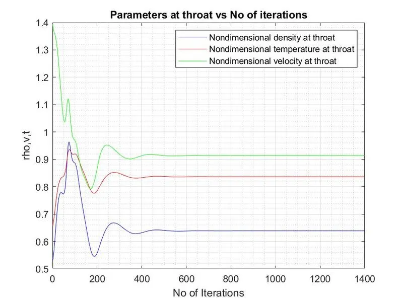
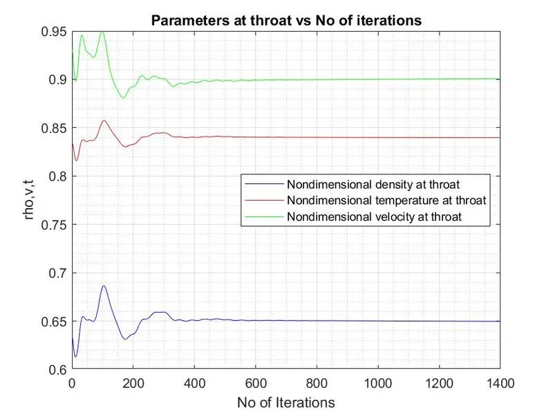
5) Timewise variation of primitive variables at throat-Nonconservative approach
6) Timewise variation of primitive variables at throat-Conservative approach
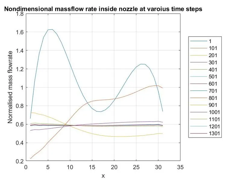
7) Nondimensional massflowrate inside nozzle for various timesteps-Nonconservative approach
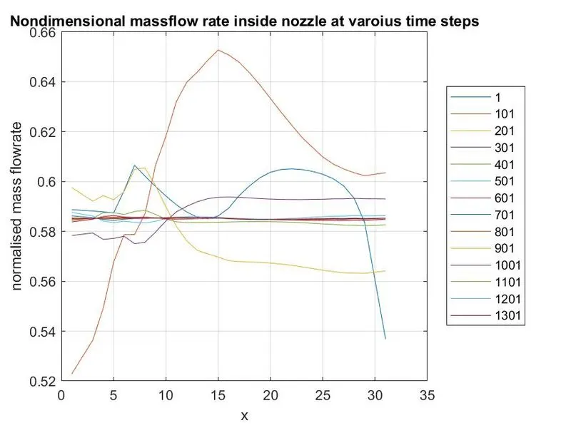
8) Nondimensional massflowrate inside nozzle for various timesteps-Conservative approach
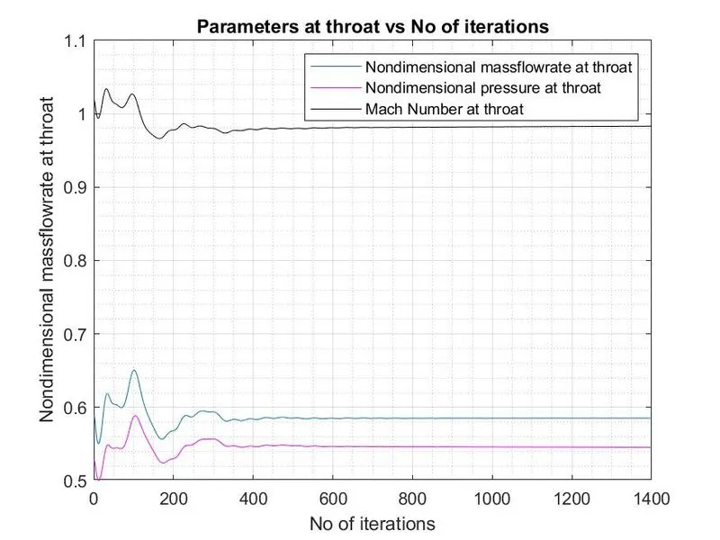
9) Timewise variation of nondimensional massfloerate,pressure & Mach Number at throat -Nonconservative approach
10) Timewise variation of nondimensional massfloerate,pressure & Mach Number at throat -Nonconservative approach
11) Comparision of nondimensional massflowrate inside nozzle between Nonconservative approach and Conservative approach
12) Variation of primitive variables at throat with varying number of nodes
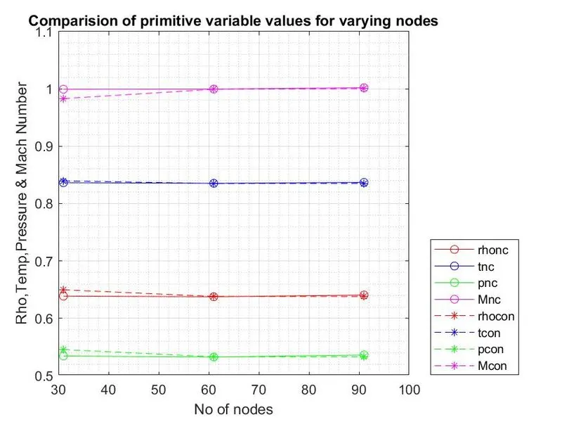
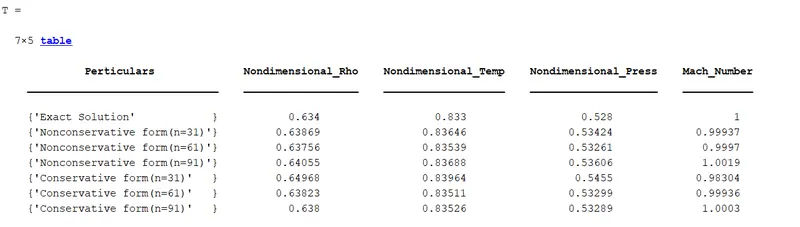
Table of exact and numerically obtained vlaues of primitive variables at throat for varying number of nodes:
Results and Observations:
- From the graph of variation of primitive variables at the throat with varying number of nodes (Graph 12) and from the table , the variation of values of primitive variables is within the accepted range of tolerance hence solution with 31 number of nodes is grid independent. Thus the results of the same can be accepted.
- The graph 1 & 2 show the area profile defined for nonconservative and conservative approaches.
- The graph of the steady state of primitive variables inside nozzle for both nonconservative and conservative approach (Graph 3 & 4), shows that results obtained from both approaches are very close to each other.
- Timewise variation of primitive variables at the throat (Graph 5,6,9 &10) shows that the changes in the values are large initially but as the number of iterations increases the steady state values are attained.
- The variation of non dimensional mass flow rate inside the nozzle is plotted for various time steps for both nonconservative and conservative approach are shown in the graph 7 & 8. From the graph it can be seen that initially the mass flow variation is large this is due to transient behaviour of the flow field variables. Then it slowly settles down to steady state.
- It has been observed that the simulation time required for the solution through conservative approach is more than the time required for the solution through nonconservative approach. It is mainly due to the extra time required to extract the primitive variable from the solution vector terms.
- The graph 11 shows the comparison of steady state non dimensional mass flow rate inside the nozzle between the nonconservative solution and conservative solution. The conservative mass flow rate is much more constant as seen from the graph than the nonconservative mass flow rate which has minute oscillations at inflow and outflow boundaries. These variations are seen on a magnified scale.
- From graph 11 it can also be seen that the conservative approach does a better job in conservation of mass in comparison with nonconservative approach. But this does not indicate the superiority of conservative approach.
- The amount by which residuals decay is used as the index of quality of the numerical algorithm in this sense the nonconservative approach performs better than conservative approach.
Conclusion:
According to the exact solution for the given set of problems and the observations and results obtained from the above Matlab code, it can be concluded that the simulation results are closely matched to the exact solution thus can be accepted within the accepted range of tolerance.
Reference:
Book: Computational Fluid Dynamics:The Basics with Application by John D. Anderson.