Week 9 - FVM Literature Review

FVM: Finite Volume Method

Finite Volume Method (FVM) is a method of discretizing a single or a set of Partial Differential Equations, in the form of approximate Algebraic expressions, which reflects conservation of one or more values. These Partial Differential Equations (PDEs) can be of a different nature, e.g. elliptic, parabolic or hyperbolic, and are used as models in many fields, including physics, biophysics, chemistry, image processing, finance, and strong reliability. They define the relationship between quantities that are part of unknown factors such as temperature, density, pressure, molar fraction, electron density or probability function, in relation to the variability within the domain (space, time) assumed.

FDM vs FVM

Finite Difference Method (FDM) discretization is based on the PDE separation form to be resolved. Each derivative is replaced by an approximate Difference formula (which can generally be obtained from an extension of the Taylor series). The computational domain is usually divided into hexahedral cells (grids), and the solution is obtained at each nodal point. FDM is easy to understand when the physical grid is Cartesian, but through curvilinear transformation, it can be extended to domains that are not easily represented by hexahedral cells. The discretization gives us a system of equations for the variable at nodal points. Once a solution is found, we get a discrete representation of the solution.

The choice of the Finite volume method (FVM) depends on the combined form of PDE to be resolved (e.g. conservation of mass, intensity, or strength). PDE is written in a form that can be solved for given Finite Volumes (or cell). The computational domain is divided into finite volumes and then governing equations are solved for each volume.

The basic advantage of FVM over FDM is that it does not require the use of structured Cartesian grids, which further enables us to avoid the conversion of the given grid into a structured grid. Given the complexity of conversion of a grid to a structured one, it saves a lot of time and effort.

FDM calculates properties on each node but FVM does it on each whole cell instead of nodes.

FDM uses Taylor series expansion and FVM uses divergence theorem.

FDM has the differential form :

`(del f_x)/(delx) = (f_(i+1) - f_i )/ (Deltax)`

FVM has the integral form :

`intint_S dxdy= ointfdy = CastArea`

Interpolation: Need and Types

In numerical analysis, Interpolation is a method of finding information where there aren't known discrete data points present.

In FVM, Interpolation is used to find the volume integrals at places other than nodal points.

Some types of Interpolation schemes are Upwind Scheme(UDS), Linear Scheme(CDS), Quadratic Upwind Interpolation Scheme(QUICK)

Upwind Interpolation

The upwind interpolation (UDS) for approximating the value of a variable at the east face of a control volume is given by

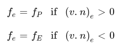
This interpolation scheme is equivalent to using a backward or forward finite difference approximation (depending on the flow direction). It is first-order accurate and is numerically diffusive with a coefficient of numerical diffusion `Gamma^(vm) = rho . (Delta x)/2`

LINEAR INTERPOLATION (CDS)

We can approximate the value of the variable at the control volume face centre by linear interpolation of the values at the two nearest computational nodes. Thus, at location 'e' on a Cartesian grid, the variable value is approximated by

`f_e = f_Elamda_e + f_p(1-lamda_e) , "where " lamda_e = (x_e - x_p) / (x_E - x_p)`

The linear interpolation is equivalent to the use of the central difference formula of the first order derivative, and hence, this scheme is also termed as the central difference scheme (CDS). This scheme is second-order accurate and may produce oscillatory solutions.

QUADRATIC UPWIND INTERPOLATION (QUICK)

A quadratic upwind interpolation (QUICK) scheme can be derived using polynomial fitting. The QUICK interpolation on a uniform Cartesian grid is given by

`phi_e = 6/8 phi_U + 3/8 phi_D -1/8 phi_(UU)`

where D, U and UU denote the downstream, the first upstream and second downstream resp.

This scheme is third-order accurate but gives oscillatory solutions as well.

FLUX LIMITERS

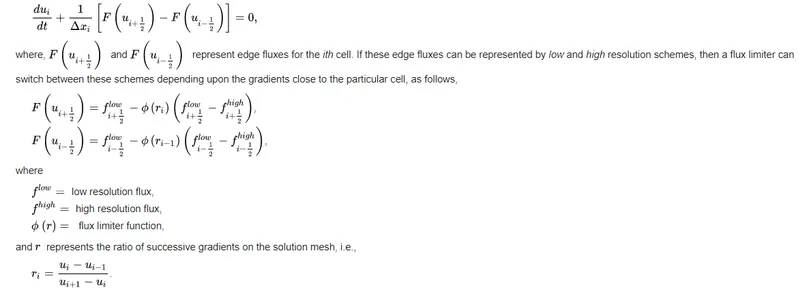
Flux limiters are used in high-resolution numerical schemes used to avoid the spurious oscillations (wiggles) which occur with high order spatial discretization schemes due to shocks, discontinuities or sharp changes in the solution domain. The use of flux limiters, together with an appropriate high-resolution scheme, makes the solutions Total Variation Diminishing (TVD).

Consider the 1D semi-discrete scheme here:

CONCLUSION

Finite Volume Method, Interpolation schemes and Flux Limiters were studied and presented here.