Week 5.1 - Mid term project - Solving the steady and unsteady 2D heat conduction problem
Solving Steady and Unsteady 2D Heat Conduction Equation
Objective: To solve two dimensional Steady and Unsteady/transient heat conduction equation by both Explicit and Implicit schemes, using point iterative techniques like Jacobi, Gauss Siedel and the Successive over-relaxation method.
Problem:
1.Temperature Boundary Conditions:
Left:400k
Top:600k
Right:800k
Bottom:900k
2. Computation Grid is a square.
3. No. of grid points in the x-direction are equal to no. of grid points in the y-direction(nx=ny).
4. Assumption that nx=ny=10.
5. All nodes will have an initial temperature of 300k except boundary points.
Theory: For function u(x,y,z,t) having spatial variables (x,y,z) and time variable t.
Heat equation :
`(del u)/(del t) = alpha ((del^2 u)/(del x^2) + (del^2 u)/(del y^2) + (del^2 u)/(del z^2) )`
where `alpha` is the diffusivity of the medium.
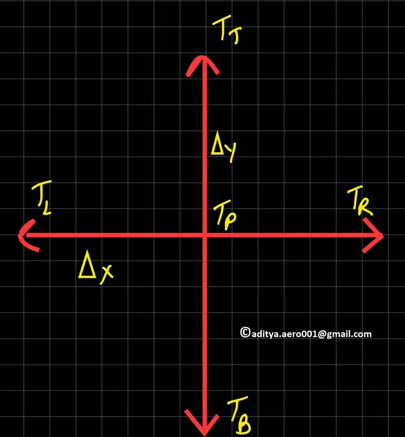
Implicit Steady State Program:
Steady State Equation Discretization:
In steady-state conduction, the net flow of the given quantity, here heat, will remain constant.
Governing Equation:
`(del^2T)/(del x^2) + (del^2T)/(del y^2) = 0`
After descretization, the above equation becomes:
`T_P = frac 1 k[ (T_L + T_R)/(Delta x^2) + (T_T + T_B)/(Delta y^2) ]`
where k = `2((Deltax^2 + Delta y^2)/(Deltax^2*Deltay^2) )`
after simplication of equation for code, it becomes:
`T_(i,j) = 0.25*(T_L + T_R + T_T + T_B)`
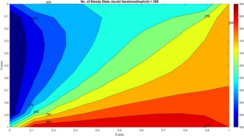
Jacobi Iteration:
%JACOBI Method
clear all
close all
clc
%INPUT
%Grid Points
nx=10;
ny=nx;
x=linspace(0,1,nx);
y=linspace(0,1,ny);
dx=x(2)-x(1);
dy=dx;
tol=1e-4; %tolerance
error=9e9;
%Boundary Conditions
T_Left=400;
T_Right=800;
T_Top=600;
T_Bottom=900;

T=300*ones(nx,ny);
T(2:ny-1,1)=T_Left;
T(2:ny-1,nx)=T_Right;
T(1,2:nx-1)=T_Top;
T(ny,2:nx-1)=T_Bottom;

%Calculating Average Temperatures at corners
T(1,1)=(T_Top+T_Left)/2;
T(nx,ny)=(T_Right+T_Bottom)/2;
T(1,ny)=(T_Top+T_Bottom)/2;
T(nx,1)=(T_Left+T_Bottom)/2;

%Assigning original values to T
T_initial=T;
T_old=T;

%Iterative Method Begins(Jacobi)
iterative_solver=1;

if iterative_solver == 1
   jacobi_iteration=1;

   while(error > tol)

       for i = 2:nx-1
           for j = 2:ny-1
               T(i,j) = 0.25*(T_old(i-1,j) + T_old(i+1,j) + T_old(i,j-1)  + T_old(i,j+1));
           end

       end
       error=max(max(abs(T_old-T)));
       T_old=T;
       jacobi_iteration=jacobi_iteration+1;
   end
end

%PLOT_Jacobi
figure(1)
contourf(x,y,T)
clabel(contourf(x,y,T))
colorbar
colormap(jet)
set(gca,'ydir','reverse')

xlabel('X-axis')
ylabel('Y-axis')
title(sprintf('No. of Steady State Jacobi Iterations(Implicit) = %d%',jacobi_iteration));
pause(0.03);
Output
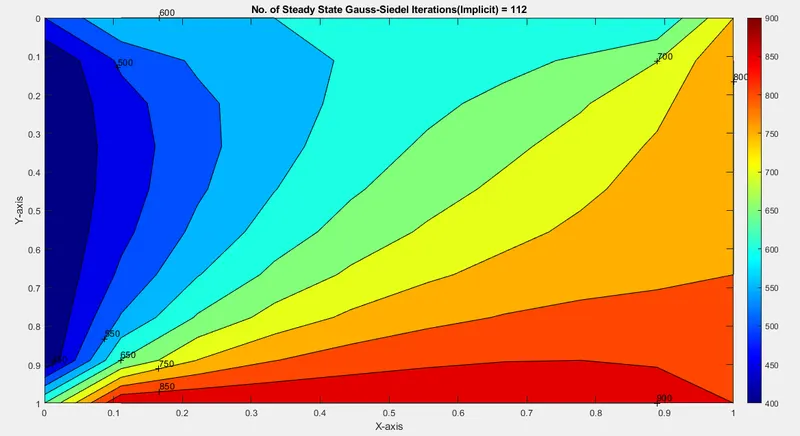
Gauss-Siedel Iteration:
%Gauss-Siedel Method
iterative_solver=2;

if iterative_solver==2
    GS_iteration=1;

    while(error > tol)

        for i = 2:nx-1
            for j = 2:ny-1

                T(i,j) = 0.25*(T(i-1,j) + T_old(i+1,j) + T(i,j-1)  + T_old(i,j+1));
            end
        end
        error=max(max(abs(T_old-T)));
       T_old=T;
       GS_iteration=GS_iteration+1;
   end
end

%PLOT_GS
figure(1)
contourf(x,y,T)
clabel(contourf(x,y,T))
colorbar
colormap(jet)
set(gca,'ydir','reverse')

xlabel('X-axis')
ylabel('Y-axis')
title(sprintf('No. of Steady State Gauss-Siedel Iterations(Implicit) = %d%',GS_iteration));
pause(0.03);
Output:
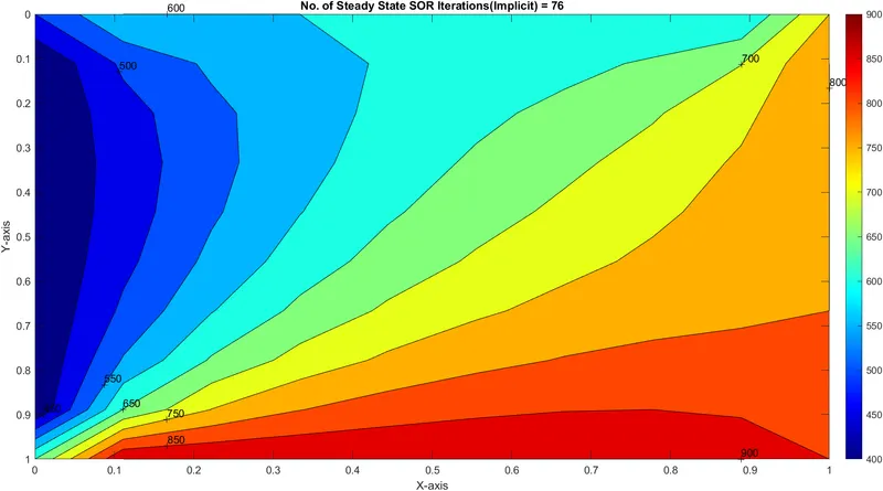
Successive Over Relaxation Method:
%SOR Method
iterative_solver=3;
omega=1.2;

if iterative_solver==3
    SOR_iteration=1;

    while(error > tol)

        for i = 2:nx-1
            for j = 2:ny-1

                T(i,j) = omega*(0.25*(T(i-1,j) + T_old(i+1,j) + T(i,j-1)  + T_old(i,j+1)))+(1-omega)*T_old(i,j);
            end
        end
        error=max(max(abs(T_old-T)));
       T_old=T;
       SOR_iteration=SOR_iteration+1;
   end
end

%PLOT_SOR
figure(1)
contourf(x,y,T)
clabel(contourf(x,y,T))
colorbar
colormap(jet)
set(gca,'ydir','reverse')

xlabel('X-axis')
ylabel('Y-axis')
title(sprintf('No. of Steady State SOR Iterations(Implicit) = %d%',SOR_iteration));
pause(0.03);
Output:
UNSTEADY-STATE 2D EQUATION IMPLICIT:
Unsteady State Equation Discretization:
Unsteady State is a condition where the net heat flow is not constant. The temperature changes at the boundary walls and inside boundary walls as well. It occurs when a source or sink is introduced into the system which causes change in temperature with time.
`(delT)/(delt) = alpha((del^2 T)/(delx^2) + (del^2 T)/(dely^2))`
Discretization:
`(T_p^(n+1) - T_p^n )/(Deltat) = alpha((T_L - 2T_P + TR)/(Deltax^2) + (T_T -2T_P + T_B)/(Deltay^2))`
Further Simplication:
`T_P^(n+1) = 1/(1+k1+k2) (T_p^n + k1(T_L+T_R)^(n+1) + k2(T_T+T_B)^(n+1))`
`k1 = alpha (Deltat)/(Deltax^2) ; k2 = alpha(Deltat)/(Deltay^2)`
`alpha` is the diffusivity term
Simplified form for code:
`T_(i,j) = 1/(1+k1+k2)(T_(i,j) + k1(T_(i-1,j) + T_(i+1,j)) + k2(T_(i,j-1) + T_(i,j+1))`
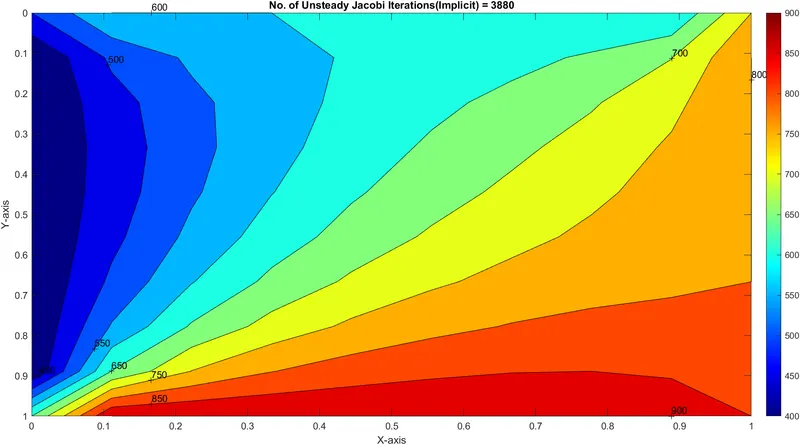
JACOBI ITERATION
%JACOBI Method

clear all
close all
clc
%INPUT
%Grid Points
nx=10;
ny=nx;
nt=1400;
x=linspace(0,1,nx);
y=linspace(0,1,ny);
dx=x(2)-x(1);
dy=dx;
tol=1e-4; %tolerance
error=9e9;
dt=1e-3;
omega=1.1;
%Boundary Conditions
T_Left=400;
T_Right=800;
T_Top=600;
T_Bottom=900;

T=300*ones(nx,ny);
T(2:ny-1,1)=T_Left;
T(2:ny-1,nx)=T_Right;
T(1,2:nx-1)=T_Top;
T(ny,2:nx-1)=T_Bottom;

%Calculating Average Temperatures at corners
T(1,1)=(T_Top+T_Left)/2;
T(nx,ny)=(T_Right+T_Bottom)/2;
T(1,ny)=(T_Top+T_Bottom)/2;
T(nx,1)=(T_Left+T_Bottom)/2;

%Assigning original values to T
T_initial=T;
T_old=T;

k1=1.1*(dt/(dx^2));
k2=1.1*(dt/(dy^2));

%Iteration Begins - JACOBI
Jacobi_iteration=1;
for k=1:nt
    error=9e9;
    while(error>tol)
        for i = 2:nx-1
            for j = 2:ny-1

                Term1=1/(1+(2*k1)+(2*k2));
                Term2=k1*Term1;
                Term3=k2*Term1;
                H=(T_old(i-1,j))+(T_old(i+1,j));
                V=(T_old(i,j-1))+(T_old(i,j+1));

                T(i,j) = (T_initial(i,j)*Term1) + H*Term2 + V*Term3;
            end
        end
        error=max(max(abs(T_old-T)));
        T_old=T;
        Jacobi_iteration=Jacobi_iteration+1;
    end
    T_initial=T;

    %PLOT Jacobi
    figure(1)
contourf(x,y,T)
clabel(contourf(x,y,T))
colorbar
colormap(jet)
set(gca,'ydir','reverse')

xlabel('X-axis')
ylabel('Y-axis')
title(sprintf('No. of Unsteady Jacobi Iterations(Implicit) = %d%',Jacobi_iteration));
pause(0.03);
end
OUTPUT:
GAUSS-SIEDEL ITERATION
%Iteration Begins - GAUSS-SIEDEL
GS_iteration=1;
for k=1:nt
    error=9e9;
    while(error>tol)
        for i = 2:nx-1
            for j = 2:ny-1

                Term1=1/(1+(2*k1)+(2*k2));
                Term2=k1*Term1;
                Term3=k2*Term1;
                H=(T(i-1,j))+(T_old(i+1,j));
                V=(T(i,j-1))+(T_old(i,j+1));

                T(i,j) = (T_initial(i,j)*Term1) + H*Term2 + V*Term3;
            end
        end
        error=max(max(abs(T_old-T)));
        T_old=T;
        GS_iteration=GS_iteration+1;
    end
    T_initial=T;

    %PLOT Gauss-Siedel
    figure(2)
contourf(x,y,T)
clabel(contourf(x,y,T))
colorbar
colormap(jet)
set(gca,'ydir','reverse')

xlabel('X-axis')
ylabel('Y-axis')
title(sprintf('No. of Gauss-Siedel Iterations(Implicit) = %d%',GS_iteration));
pause(0.03);
end
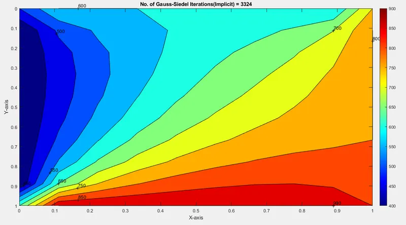
OUTPUT:
SUCCESSIVE-OVER RELAXATION ITERATION
%Iteration Begins - S.O.R
SOR_iteration=1;
for k=1:nt
    error=9e9;
    while(error>tol)
        for i = 2:nx-1
            for j = 2:ny-1

                Term1=1/(1+(2*k1)+(2*k2));
                Term2=k1*Term1;
                Term3=k2*Term1;
                H=(T(i-1,j))+(T_old(i+1,j));
                V=(T(i,j-1))+(T_old(i,j+1));

                T(i,j) = (T_initial(i,j)*Term1) + H*Term2 + V*Term3;
                T_end(i,j)=((1-omega)*T_old(i,j))+(T(i,j)*omega);
            end
        end
        error=max(max(abs(T_old-T)));
        T_old=T_end;
        SOR_iteration=SOR_iteration+1;
    end
    T_initial=T_end;

    %PLOT SOR
    figure(1)
contourf(x,y,T)
clabel(contourf(x,y,T))
colorbar
colormap(jet)
set(gca,'ydir','reverse')

xlabel('X-axis')
ylabel('Y-axis')
title(sprintf('No. of S.O.R Iterations(Implicit) = %d%',SOR_iteration));
pause(0.03);
end
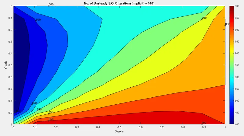
OUTPUT:
UNSTEADY STATE 2D EQUATION EXPLICIT
Unsteady State Equation Discretization:
Unsteady State is a condition where the net heat flow is not constant. The temperature changes at the boundary walls and inside boundary walls as well. It occurs when a source or sink is introduced into the system which causes change in temperature with time.
`(delT)/(delt) = alpha((del^2 T)/(delx^2) + (del^2 T)/(dely^2))`
Discretization:
`(T_p^(n+1) - T_p^n )/(Deltat) = alpha((T_L - 2T_P + TR)/(Deltax^2) + (T_T -2T_P + T_B)/(Deltay^2))`
Further Simplification:
`T_p^(n+1) = T_p^n + k1(T_L - 2T_P +T_R)^n + k2(T_T - 2T_P +T_B)^n`
`k1 = alpha (Deltat)/(Deltax^2) ; k2 = alpha(Deltat)/(Deltay^2)`
`alpha` is the diffusivity term
Simplified form for code:
`T_(i,j) = T_(i,j) + k1(T_(i-1,j) - 2T_(i,j) + T_(i+1,j)) + k2(T_(i,j-1) -2T_(i,j) + T_(i,j+1) )`
Code for Explicit scheme Unsteady Equation using SOR :
%Solving Unsteady State 2D Heat equation EXPLICITLY using SOR iterative method%

clear all
close all
clc
%INPUT
%Grid Points
nx=10;
ny=nx;
nt=1400;
x=linspace(0,1,nx);
y=linspace(0,1,ny);
dx=x(2)-x(1);
dy=dx;
tol=1e-4; %tolerance
error=9e9;
dt=1e-3;
omega=1.1;
%Boundary Conditions
T_Left=400;
T_Right=800;
T_Top=600;
T_Bottom=900;

T=300*ones(nx,ny);
T(2:ny-1,1)=T_Left;
T(2:ny-1,nx)=T_Right;
T(1,2:nx-1)=T_Top;
T(ny,2:nx-1)=T_Bottom;

%Calculating Average Temperatures at corners
T(1,1)=(T_Top+T_Left)/2;
T(nx,ny)=(T_Right+T_Bottom)/2;
T(1,ny)=(T_Top+T_Bottom)/2;
T(nx,1)=(T_Left+T_Bottom)/2;

%Assigning original values to T
T_initial=T;
T_old=T;

iterative_solver=1;
k1=1.1*(dt/(dx^2));
k2=1.1*(dt/(dy^2));

%Iteration Begins - SOR
if iterative_solver==1
    steady_explicit=1;
for k=1:nt
    error=1;
    while(error>tol)
        for i = 2:nx-1
            for j = 2:ny-1

                Term1=T_old(i,j);
                Term2=k1*(T_old(i+1,j)-(2*T_old(i,j))+T_old(i-1,j));
                Term3=k2*(T_old(i,j+1)-2*T_old(i,j)+T_old(i,j-1));
                T(i,j)=Term1 + Term2 + Term3;

            end
        end
        error=max(max(abs(T_old-T)));
        T_old=T;
        steady_explicit=steady_explicit+1;
    end
end
end


%PLOT SOR
figure(1)
contourf(x,y,T)
clabel(contourf(x,y,T))
colorbar
colormap(jet)
set(gca,'ydir','reverse')

xlabel('X-axis')
ylabel('Y-axis')
title(sprintf('No. of SOR(Explicit) = %d%',steady_explicit));
pause(0.03);
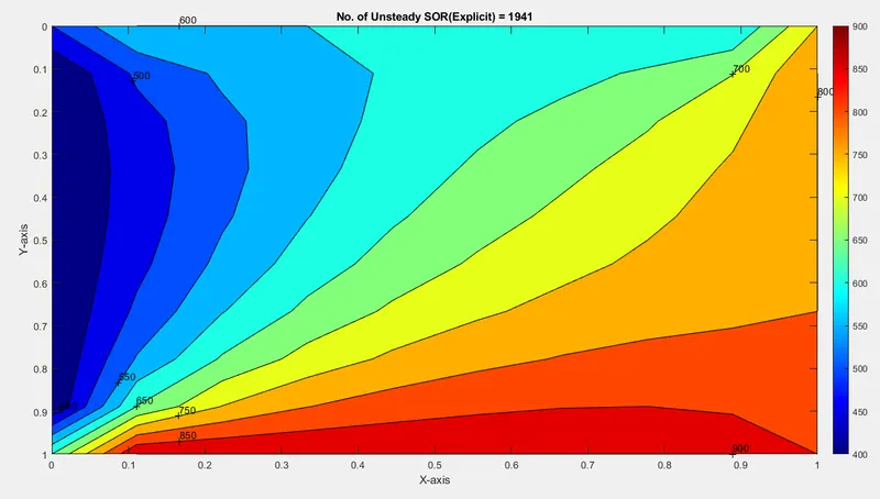
OUTPUT:
| Analysis Type and Scheme | Iterative Method | No. of convergent Iterations |
| Steady State - IMPLICIT | Jacobi | 208 |
| Steady State - IMPLICIT | Gauss Siedel | 112 |
| Steady State - IMPLICIT | Successive Over Relaxation | 76 |
| Unsteady State - IMPLICIT | Jacobi | 3880 |
| Unsteady State - IMPLICIT | Gauss Siedel | 3324 |
| Unsteady State - IMPLICIT | Successive Over Relaxation | 1401 |
| Unsteady State - EXPLICIT | Successive Over Relaxation | 1941 |
CONCLUSION:
Hereby, from above analysis and results, we can conclude:
1. In terms of number of iterations to converge the solution, SOR<G.S<Jacobi.
2. In comparison of Steady state and Unsteady state analysis, steady state analysis takes less time and iterations and converge.
3. Among all three iterative techniques, Successive Over Relaxation is most effective in both Implicit and Explicit schemes, as it takes least time and iterations to converge the solution.