Week 7 - Simulation of a 1D Super-sonic nozzle flow simulation using Macormack Method
OBJECTIVE: The objective is to simulate Quasi 1D Nozzle flow through solving Conservative and Non-Conservative governing equations using MacCormack Method.
PROBLEM STATEMENT: Determine the steady-state temperature distribution for the flow field variables and compare the results of the two forms by plots of:
1. Steady-State variation of the primitive variables across the nozzle.
2. Unsteady-State variation of the primitive variables across the nozzle.
3. Variation of Mass flow rate inside nozzle at different time steps during the Time Marching process.
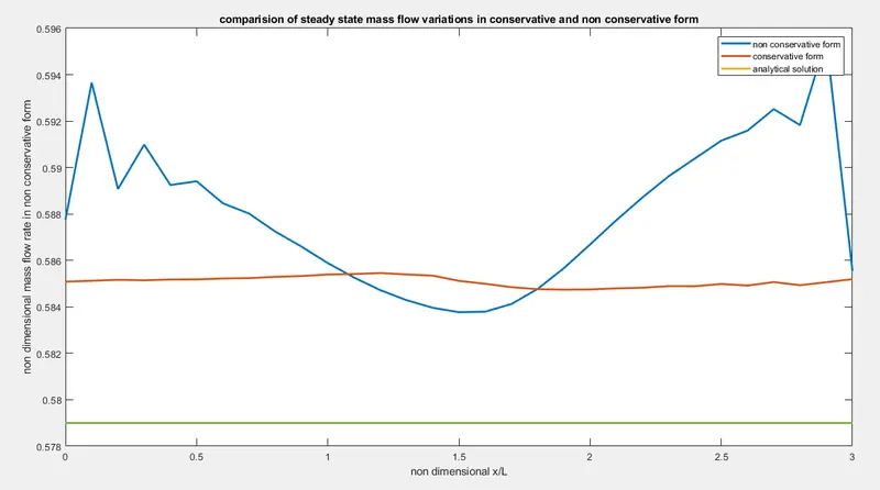
4. Comparison of normalized mass flow rate distribution of both forms.
5. Grid Dependency test to check which method first attains the steady-state.
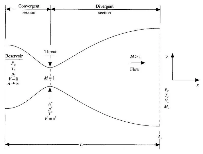
THEORY: We assume the flow inside C-D Nozzle to be Steady and Isentropic. The Inlet receives the flow, which goes from Inlet to Nozzle, from a reservoir where the Pressure and Temperature are Po and To respectively and has a cross-sectional area of A `rightarrow` `infty` , for which Velocity V `rightarrow``infty` . `P_o` and `T_o` are stagnation values and Flow expansion happens isentropically.
As for every Nozzle problem, we will focus on three sections of the Nozzle flow problem :
1.Subsonic Section which is the Convergent section of Nozzle, where Mach no. < 1.
2.The Throat, which is a Sonic region where Mach no. = 1, denoted by '*' values in figure.
3.Supersonic Section which is the Divergent section of Nozzle, where Mach no. > 1.
Governing Equation for Analytical Solution :
Continuity : `rho_1V_1A_1 = rho_2V_2A_2`
Momentum : `p_1A_1 + rho_1V_1^2A_1 + int_(A1)^(A2) pdA = p_2A_2 + rho_2V_2^2A_2`
Energy : `h_1 + V_1^2/2 = h_2 + V_2^2/2`
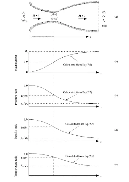
Solution of the above Equations produces the below results : (John D Anderson)
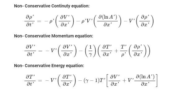
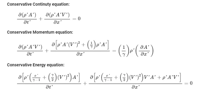
Governing Equation for Numerical Solution :
Non-Dimensional Quantities :
Temperature : `T' = T/T_o`
Density : `rho' = rho/rho_o`
Length : `x' = x/x_o`
Velocity : `V' = V/a_o` , where `a_o` is the local velocity of sound `a_o = sqrt(gammaRT_o`
Time : `t' = t/(L/a_o)` , where `L/a_o` is the characteristic time scale
Area : `A' = A/A_o`
MacCormack Method :
MacCormack method is a technique to discretize numerical solution. It is a variation of two steps Lax-Wendroff scheme, having a much simpler application.
Predictor Step :
In this step, we estimate the value of u and this is the reason why this step is called the Predictor step. Value of u at time level 'n+1' is calculated `(u_i^(n+1))` using forward differencing method and `Delta t` as time step.
Corrector Step :
In this step, we correct the value of u obtained in predictor step and this is the reason why this step is called the Corrector step. Value of u at time level 'n+1' is calculated `(u_i^(n+1))` using backward differencing method and; `(Delta t)/2` as time step`
MAIN PROGRAM :
clear all
close all
clc

%INPUTS
L=3;
n=31;
dx=L/(n-1);
C=0.5;
nt=1400;
gamma=1.4;
%N/D stands for Non-Dimensional


%non-conservative governing equations solution
tic
[x,dt,rho,v,T,p,M,flow_rate_n,nt_grid,n_iter]=non_conservative_form(L,n,C,dx,nt);
toc
time_nc=toc;
fprintf('time taken for solution to converge in non conservative form = %0.4gs', time_nc)


%conservative governing equations solution
tic
[dt,rho,T,p,M,v,flow_rate_c,m_analytical,cn_iter,tolerance]=conservative_form(L,n,C,dx,gamma,nt);
toc
time_con=toc;
fprintf('time taken for solution to converge in conservative form = %0.4gs', time_con)


figure(7)
plot(x,flow_rate_n,'Linewidth',2)
hold on
plot(x,flow_rate_c,'Linewidth',2)
hold on
plot(x,m_analytical,'Linewidth',2)
legend('non conservative form','conservative form','analytical solution')
xlabel('non dimensional x/L','Fontsize',11);
ylabel('non dimensional mass flow rate in non conservative form','Fontsize',11)
title(sprintf(['comparision of steady state mass flow variations in conservative and non conservative form']))


figure(8)
%bar graph of convergence rate
no_of_iterations = [n_iter cn_iter];
bar(no_of_iterations,'g')

set(gca,'xticklabel',{'non conservative form','conservative form'});
ylabel('no. of iterations ');
title(sprintf(['No. of iterations to achieve steady state for tolerance of %g'],tolerance));
legend('No. of iterations');


%Plotting steady state values of flow field

figure(2)
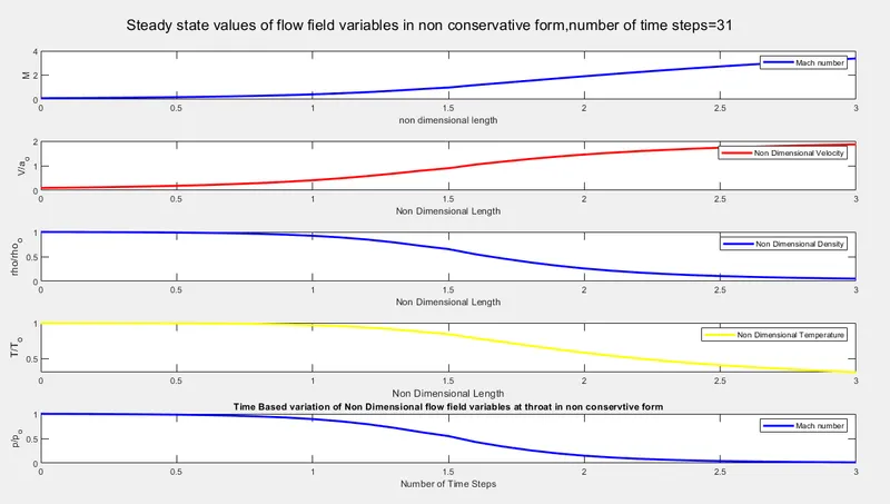
sgtitle(sprintf('Steady state values of flow field variables in non conservative form,number of time steps=%d',n))
subplot(5,1,1)

plot(x,M,'b','Linewidth',2);
xlabel('non dimensional length');
ylabel('M');
legend('Mach number')

subplot(5,1,2)
plot(x,v,'r','Linewidth',2);
xlabel('Non Dimensional Length');
ylabel('V/a_o');
legend('Non Dimensional Velocity')

subplot(5,1,3)
plot(x,rho,'b','Linewidth',2);
xlabel('Non Dimensional Length');
ylabel('rho/rho_o','Fontsize',10);
legend('Non Dimensional Density')

subplot(5,1,4)
plot(x,T,'y','Linewidth',2);
xlabel('Non Dimensional Length','Fontsize',10);
ylabel('T/T_o','Fontsize',10);
legend('Non Dimensional Temperature')

subplot(5,1,5)
plot(x,p,'b','Linewidth',2);
xlabel('Non Dimensional Length');
ylabel('p/p_o');
legend('Non Dimensional Pressure')


%FUNCTION FOR NON CONSERVATIVE FORM OF GOVERNING EQUATIONS

function[x,dt,rho,v,T,p,M,flow_rate_n,nt_grid,n_iter]=non_conservative_form(L,n,C,dx,nt)
%INITIAL CONDITIONS
x=linspace(0,L,n);
rho=1-0.3146*x;
T=1-0.2314*x;
v=(0.1+1.09*x).*T.^0.5;
A=1+2.2*(x-1.5).^2;
gamma=1.4;
throat=(n+1)/2;
nt_grid=linspace(1,nt,nt);
initial_flow=rho.*v.*A;
flow_rate_old=0;
tolerance=1e-4;
error=999;
n_iter=1;

%Analytical mass flow rate
m_analytical=0.579*ones(n);
%Calculation minimum dt at all nodes


for k=1:nt
    rho_old=rho;
    T_old=T;
    v_old=v;
    for m=1:n
    dt_x(m)=C*(dx/(T(m)^0.5+v(m)));
    end

dt=min(dt_x);

    %PREDICTOR METHOD
    for i=2:n-1
        dvdx=(v(i+1)-v(i))/dx;
        drhodx=(rho(i+1)-rho(i))/dx;
        dT_dx=(T(i+1)-T(i))/dx;
        dlogA_dx=(log(A(i+1))-log(A(i)))/dx;

        %CONTINUITY EQUATION
        drhodt_p(i)= -rho(i)*dvdx-rho(i)*v(i)*dlogA_dx-v(i)*drhodx;

        %MOMENTUM EQUATION
        dvdt_p(i)=-v(i)*dvdx- (1/gamma)*(dT_dx+(T(i)/rho(i))*drhodx);

        %ENERGY EQUATION
        dTdt_p(i)= -v(i)*dT_dx - (gamma-1)*T(i)*(dvdx + (v(i)*dlogA_dx));
    end

    %Predictor Solution step update
for i=2:n-1

    rho(i)=rho(i)+drhodt_p(i)*dt;
    v(i)=v(i)+dvdt_p(i)*dt;
    T(i)=T(i)+dTdt_p(i)*dt;
end

%CORRECTOR STEP
for i = 2:n-1
    dvdx=(v(i)-v(i-1))/dx;
    drhodx=(rho(i)-rho(i-1))/dx;
    dT_dx=(T(i)-T(i-1))/dx;
    dlogA_dx=(log(A(i))-log(A(i-1)))/dx;

        %CONTINUITY EQUATION
        drhodt_c(i)= -rho(i)*dvdx-rho(i)*v(i)*dlogA_dx-v(i)*drhodx;

        %MOMENTUM EQUATION
        dvdt_c(i)=-v(i)*dvdx- (1/gamma)*(dT_dx+(T(i)/rho(i))*drhodx);

        %ENERGY EQUATION
        dTdt_c(i)= -v(i)*dT_dx - (gamma-1)*T(i)*(dvdx + (v(i)*dlogA_dx));
end


    % Computation of average time derivatives

    dvdt=0.5*(dvdt_p+dvdt_c);
    dTdt=0.5*(dTdt_p+dTdt_c);
    drhodt=0.5*(drhodt_p+drhodt_c);

    % Final Step Update
    for i=2:n-1
        rho(i)=rho_old(i)+drhodt(i)*dt;
        v(i)=v_old(i)+dvdt(i)*dt;
        T(i)=T_old(i)+dTdt(i)*dt;
    end

    % Inlet Boundary Condition
    v(1)=2*v(2)-v(3);

    % Outlet Boundary Condition
    v(n)=2*v(n-1) - v(n-2);
    rho(n)=2*rho(n-1) - rho(n-2);
    T(n)=2*T(n-1) - T(n-2);

    %Calculation of Pressure,Mach No. and Mass flow rate
    p=rho.*T;
    M=(v./((T).^0.5));
    flow_rate_n=rho.*v.*A;


    %Capturing flow field values at throat for each time step

    rho_throat(k)=rho(throat);
    v_throat(k)=v(throat);
    T_throat(k)=T(throat);
    p_throat(k)=p(throat);
    M_throat(k)=M(throat);
    flow_rate_throat(k)=flow_rate_n(throat);

    error = max(abs(flow_rate_n-flow_rate_old));
    if error>tolerance
        n_iter=n_iter+1;
        flow_rate_old=flow_rate_n;
    end


    figure(1)
    %Non dimensional mass flow distribution across the nozzle at different
    %time steps compared with analytical mass flow rate solution

    if k == 50
        plot(x,flow_rate_n,'Linewidth',2)
        hold on
    else if k == 100
        plot(x,flow_rate_n,'Linewidth',2)
        hold on
    else if k == 200
        plot(x,flow_rate_n,'Linewidth',2)
        hold on
    else if k == 500
        plot(x,flow_rate_n,'Linewidth',2)
        hold on
    else if k == 700
        plot(x,flow_rate_n,'Linewidth',2)
        hold on

        plot(x,m_analytical,':')
        hold on

        plot(x,initial_flow,'--')

% M_throat(k)=M(16);
% rho_throat(k)=rho(16);
% v_throat(k)=v(16);
% T_throat(k)=T(16);


    legend('50Deltat','100Deltat','200Deltat','500Deltat','700Deltat','Analytical solution','Initial flow rate');
    title('Mass flow distribution(non dimensional) across the nozzle at different time steps');
    xlabel('Non Dimensional x/L');
    ylabel('Mass flow rate in non conservative form','Fontsize',11);
        end
        end
        end
        end
    end


end
M_throat(k)=M(16);
    rho_throat(k)=rho(16);
    v_throat(k)=v(16);
    T_throat(k)=T(16);
    p_throat(k)=p(16);

    figure(3)
%Time dependent variation of flow field variables and mach number at throat
plot(nt_grid,M_throat,'Linewidth',2)
hold on
plot(nt_grid,rho_throat,'Linewidth',2)
hold on
plot(nt_grid,v_throat,'Linewidth',2)
hold on
plot(nt_grid,T_throat,'Linewidth',2)
hold on


end

%Function for Conservative form of Governing equation solution
function[dt,rho,T,p,M,v,flow_rate,m_analytical,cn_iter,tolerance]=conservative_form(L,n,C,dx,gamma,nt)

%Initial Conditions
x=linspace(0,L,n);
A=1+2.2*(x-1.5).^2;
throat=(n+1)/2;
nt_grid=linspace(1,nt,nt);
%Mass flow-rate-Analytical
m_analytical=0.579*ones(n);
cn_iter=1;
%Mass flow rate at t=0
U2_i=0.59;
flow_rate_old=0;
tolerance=1e-4;
error=999;
for i=1:n
    if x(i)>=0 && x(i)<0.5
        rho(i)=1.0;
        T(i)=1.0;
    else if x(i)>=0.5 && x(i)<=1.5
            rho(i)=1-(0.366*(x(i)-0.5));
            T(i)=1-(0.167*(x(i)-0.5));
        else if x(i)>=1.5 && x(i)<=3.5
             rho(i)=0.634-(0.3879*(x(i)-1.5));
             T(i)=0.833-(0.35077*(x(i)-1.5));

        end
    end
    end
end

%Solution Vectors U1 U2 and U3 which are not primitive variables

for j=1:n

    v(j)=U2_i/(rho(j)*A(j));
    U1(j)=rho(j)*A(j);
    U2(j)=rho(j)*A(j)*v(j);
    U3(j)=rho(j)*A(j)*((T(j)/(gamma-1))+(0.5*gamma*v(j)^2));
end

%Calculating minimum of dt at all nodes
for m=1:n
    dt_x(m)=C*(dx/(T(m)^(0.5)+v(m)));
end

%Time step
dt=min(dt_x);

U2_initial=U2;

for k=1:nt

    U1_old=U1;
    U2_old=U2;
    U3_old=U3;


    %Flux terms which are functions of solution vector
    F1=U2;
    F2=((U2.^2)./(U1))+(((gamma-1)/gamma).*(U3-((gamma/2).*(((U2.^2)./U1)))));
    F3=((gamma.*U2.*U3)./U1) - (gamma.*(gamma-1)/2)*((U2.^3)./U1.^2);

    for i = 2:n-1
        dF1_dx=(F1(i+1) - F1(i))/dx;
        dF2_dx=(F2(i+1) - F2(i))/dx;
        dF3_dx=(F3(i+1) - F3(i))/dx;

        %PREDICTOR STEP

        %Continuity Equation
        dU1_dt_p(i) = -dF1_dx;

        %Momentum Equation
        J2(i)= ((1/gamma)*rho(i)*T(i)*((A(i+1)-A(i))/dx));
        dU2_dt_p(i) = -dF2_dx+J2(i);

        %Energy
        dU3_dt_p(i) = -dF3_dx;


        %Solution update of solution vectors
        U1(i) = U1(i) + dU1_dt_p(i)*dt;
        U2(i) = U2(i) + dU2_dt_p(i)*dt;
        U3(i) = U3(i) + dU3_dt_p(i)*dt;
    end

    %Updation on initial values
    rho = U1./A;
    v = U2./U1;
    T = (gamma-1).*((U3./U1)-(0.5*gamma.*v.^2));
    p=rho.*T;

    %Computing new set of values using predicted values
    F1=U2;
    F2=((U2.^2)./(U1))+(((gamma-1)/gamma).*(U3-((gamma/2).*(((U2.^2)./U1)))));
    F3=((gamma.*U2.*U3)./U1) - (gamma.*(gamma-1)/2).*((U2.^3)./U1.^2);

    %CORRECTOR STEP
    %Calculating derivative terms via backward difference for corrector-method
    for j = 2:n-1
        dF1_dx = (F1(j)-F1(j-1))/dx;
        dF2_dx = (F2(j)-F2(j-1))/dx;
        dF3_dx = (F3(j)-F3(j-1))/dx;

        %Continuity Equation
        dU1_dt_c(j)= -dF1_dx;

        %Momentum Equation
        J2(j)=((1/gamma)*rho(j)*T(j)*((A(j)-A(j-1))/dx));
        dU2_dt_c(j)= -dF2_dx + J2(j);

        %Energy Equation
        dU3_dt_c(j)=-dF3_dx;
    end

%Average Values

dU1_dt_avg = 0.5*(dU1_dt_p + dU1_dt_c);
dU2_dt_avg = 0.5*(dU2_dt_p + dU2_dt_c);
dU3_dt_avg = 0.5*(dU3_dt_p + dU3_dt_c);

%Final corrected values

for m = 2:n-1
    U1(m)= U1_old(m)+ dU1_dt_avg(m)*dt;
    U2(m)= U2_old(m)+ dU2_dt_avg(m)*dt;
    U3(m)= U3_old(m)+ dU3_dt_avg(m)*dt;
end

%Inlet Boundary Conditions
U1(1)=rho(1)*A(1);
U2(1)=2*U2(2)-U2(3);
v(1)=U2(1)/(rho(1)*A(1));
U3(1)=U1(1)*((T(1)/(gamma-1))+((gamma*0.5)*v(1)^2));

%Outlet conditions
U1(n)= 2*U1(n-1) - U1(n-2);
U2(n)= 2*U2(n-1) - U2(n-2);
U3(n)= 2*U3(n-1) - U3(n-2);

%Update of primitive variables
rho = U1./A;
v = U2./U1;
T = (gamma-1).*((U3./U1)-(0.5*gamma.*v.^2));

%Calculating pressure(p),Mach no.(M), mass flow rate
p=rho.*T;
M=(v./((T).^0.5));
flow_rate=rho.*v.*A;

%Capturing flow field values at each time step
rho_throat(k)=rho(throat);
v_throat(k)=v(throat);
T_throat(k)=T(throat);
p_throat(k)=p(throat);
M_throat(k)=M(throat);
flow_rate_throat(k)=flow_rate(throat);


error = max(abs(flow_rate-flow_rate_old));
if error > tolerance
    cn_iter=cn_iter+1;
    flow_rate_old=flow_rate;
end

%non dimensional mass flow distribution across the nozzle at different
%time steps, compared with analytical mass flow rate solution

figure(4)

if k == 50
    plot(x, flow_rate,'Linewidth',2);
    hold on
else if k == 100
        plot(x, flow_rate,'Linewidth',2);
    hold on
    else if k == 200
            plot(x,flow_rate,'Linewidth',2);
            hold on
        else if k == 500
                plot(x,flow_rate,'Linewidth',2);
                hold on
            else if k == 700
                    plot(x,flow_rate,'Linewidth',2);
                    hold on
                    plot(x,m_analytical,':');
                    hold on
                    plot(x,U2_initial,'--');

                    legend('50Deltat','100Deltat','200Deltat','400Deltat','700Deltat','analytical solution','initial flow rate');
                    title('non dimensional mass flow distribution across the nozzle at different time steps before steady state coservative form');
                    xlabel('non dimensional x/L','Fontsize',11);
                    ylabel('Mass flow rate conservative','Fontsize',11);
                    axis([0 3 0.5 1])
                end
            end
        end
    end
end
end

%Plotting steady state values of flow field variables at each node

figure(5)
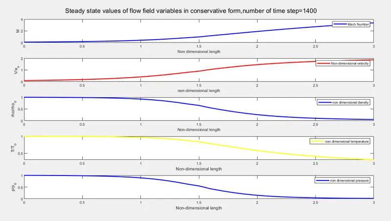
sgtitle(sprintf('Steady state values of flow field variables in conservative form,number of time step=%d',k))
subplot(5,1,1)
plot(x,M,'b','Linewidth',2);
xlabel('Non dimensional length');
ylabel('M');
legend('Mach Number')

subplot(5,1,2)
plot(x,v,'r','Linewidth',2);
xlabel('non-dimensional length');
ylabel('V/a_o');
legend('Non-dimensional velocity')

subplot(5,1,3)
plot(x,rho,'b','Linewidth',2);
xlabel('Non-dimensional length');
ylabel('rho/rho_o','Fontsize',10);
legend('non dimensional density')

subplot(5,1,4)
plot(x,T,'y','Linewidth',2);
xlabel('Non-dimensional length','Fontsize',10);
ylabel('T/T_o','Fontsize',10);
legend('non dimensional temperature')

subplot(5,1,5)
plot(x,p,'b','Linewidth',2);
xlabel('Non-dimensional length','Fontsize',10);
ylabel('p/p_o','Fontsize',10);
legend('non dimensional pressure')

%Time-wise variation of flow field variables & Mach no. at nozzle throat
figure(6)
plot(nt_grid,M_throat,'Linewidth',2)
hold on
plot(nt_grid,rho_throat,'Linewidth',2)
hold on
plot(nt_grid,v_throat,'Linewidth',2)
hold on
plot(nt_grid,T_throat,'Linewidth',2)
hold on
plot(nt_grid,p_throat,'Linewidth',2)
hold on

legend('Mach number','N/D density(rho/rho_o)','N/D velocity(v/a)','N/D Temperature(T/T_o)','N/D pressure(p/p_o)')
xlabel('Number of time steps')
axis([0 1400 0.5 1.2])
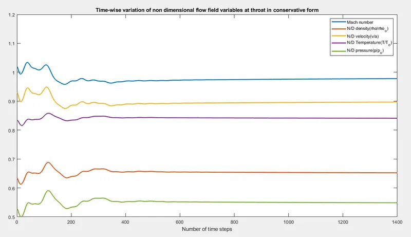
title('Time-wise variation of non dimensional flow field variables at throat in conservative form')

end
RESULTS :
Plots:
1. Steady-State values of flow field variables in non-conservative form
2. Steady-State values of flow field variables in conservative form
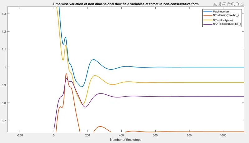
3. Timewise Variation of flow field variables at Throat in Non-Conservative and Conservative
4. Non Dimensional Mass Flow Rate distribution at different time steps in both Non-Conservative and Conservative Forms
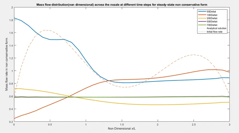
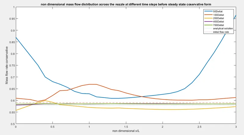
5. Comparison of Conservative and Non-Conservative forms for attaining steady-state for a tolerance of 1e-4
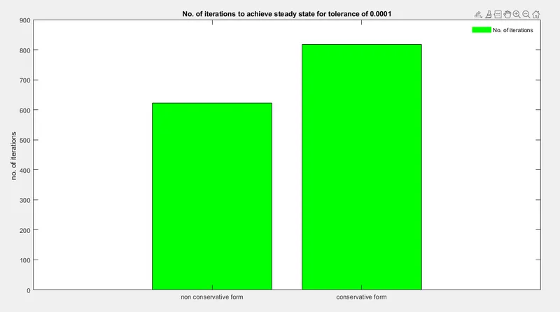
6. Comparison of Non-Dimensional Mass Flow Rate variation of Conservative and Non-Conservative solution with Analytical Solution
Grid Dependency Check :
| M | `(rhoast)/rho` | `(Tast)/T` | `(past)/p` | |
| Analytical Solution | 1 | 0.634 | 0.833 | 0.528 |
| Numerical Solution for Non-Conservative form(31 grid points) | 0.9994 | 0.6387 | 0.8365 | 0.5342 |
| Numerical Solution for Conservative form(31 grid points) | 0.978 | 0.6524 | 0.841 | 0.5487 |
| Numerical Solution for Non-Conservative form(61 grid points) | 0.9998 | 0.6377 | 0.8354 | 0.5327 |
| Numerical Solution for Conservative form(61 grid points) | 0.9979 | 0.6391 | 0.8355 | 0.534 |
Observing the above results, we can draw following insights :
1. Comparing Conservative form to Non Conservative form, it is evident that Non-Conservative is closer to Analytical solution.
2. After doubling the grid points, the Non-Conservative form is still more closer to Analytical solution than Conservative form.
3. After doubling the grid points, there isn't much change in Non-Consevative solution, but the Conservative solution becomes more accurate and closer to the Analytical solution.
From the above insights, we can conclude that :
a) Numerical solution of Non-Conservative form is more accurate than Conservative form.
b) The Non-Conservative form is Grid Independent, however, the Conservative form can concluded as Grid Dependent.
CONCLUSION
1. Conservative form gives a better Mass Flow rate distribution.
2. Non-Conservative form gives more accurate solution.
3. Numerical solution of Non-Coservative is Grid Independent but for Conservative form, it is Grid Dependent