Week 9 - FVM Literature Review

                                                                                                    FVM Literature Review

AIM:-

To describe the need for interpolation schemes and flux limiters in FVM

THEORY:-

Discretization is the process of converting partial Diffrential Equation in to Algeberic form.The whole idea behind discretization is to get the solution at discrete points.

Methods of Discretization:-

1. Finite Difference Method:- Simple, Straightforward to apply and Structured Grids.
2. Finite Element Method:- applied to any Geometries.
3. Finite Volume Method:- Conservative and applied to any Geometries

FINITE VOLUME METHOD:-

In case of FVM the problem domain is divided in to number of non-overlapping control volume called Finite volume. Finite volume is based upon the approximate solution of the integral form of the conservation equation. The integral form of conservation law for a control volume involves both surface and volume integral.

The diffrential equation is integrated over each control volume. Piecewise profiles expressing the variation of the unknown between the grid points are used to evaluvate the required integrals. integral occuring in the conservation equations are evaluated using the function values at computational nodes.

Finite volume refers to small volume surrounding each node point on a mesh. In FVM equations are written in an entire volume and no assumptions were made over the shape of the volume. Inside this particular volume all the flow and flow quantities are conserved.

                                   

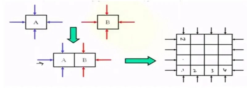
Consider 2 particular finite volumes A and B as shown above. The flux is going in and out of the volume To get the complete set of domain or the grid all the indivdual volumes like A and B are combined.

Features of FVM:-

1. FVM can accomodate any type of grid and hence it is naturally suitable for any type of grid.
2. Unstructured grid generation methods and mesh partioning techniques developed for Finite Element Method can be directly used in FVM.

TYPES OF FINITE VOLUME GRIDS:-

1. Cell centred approach:-

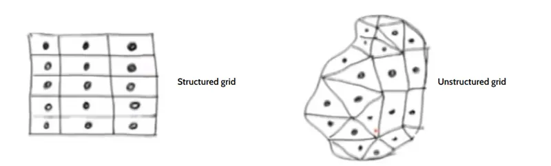
 Control volumes are defined by a suitable grid and computational nodes are assigned at the control volume centre. It can be applied for both structured and unstructured grids. Cell centred nodal value represents mean over the Control volume. This approach is the most commonly used Finite volume Method.

                                 

2. Face centred approach:-

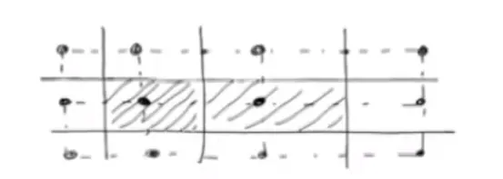
 Nodal locations are defined first and control volumes are then constructed around them so that the control volume faces lie in the midway between the nodes. It can only be used with structured grids.

                                      

Approximation of Surface integral:-

 Net flux through the control volume boundaries is the sum of the integral over the control volume faces. where 'f' is the component of the convective or diffusive flux in the direction normal to the control volume.

`int_s f ds = sum_kint_(sk) f ds`

STEPS IN FV DISCRETIZATION:-

1. Obtain the governing Equation in its integral form
2. Apply Gauss Divergence Theorem
3. Come up with suitable methods to calculate flux terms

Consider the 1D Steady state heat conduction equation

`(partial/(partialx)(alpha(partialT)/(partialx))+S = 0`

S ---> Source term   `(partialT)/(partialx)`----> Temprature gradient along x direction  `alpha`----> Thermal Diffusivity

     

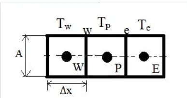
The growing equation is valid at every point in the domain which means it is valid in the entire control volume

Multiplying the governing equation by 'dv' and integrating it

  

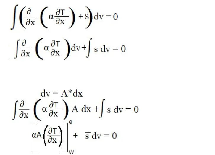
`overline S` is the average value of the source term(s)

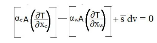
`alpha` is kind of constant and not a function of temperature

`alpha_e and alpha_w` are used for consistency

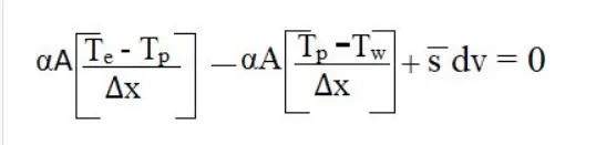
if the source term added is the function of temprature we have to linearize it

`overlineS = S_u+S_PT_P`

`[Heat flux]_(out) - [Heat flux]_(in) + sourceterm = 0`

Types of scheme:-

1. Gradient scheme 
2. Interpolation scheme

1.Gradient scheme:-

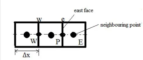
For calculating the temprature gradient at east face we use neighbouring point temprature to numerically represent temprature gradient and this is referred as Gradient Scheme

2. Interpolation scheme:-

The approximations of surface and volume integrals require values of the variables at locations other than computational nodes of the control Volume. Values of these locations are obtained using interpolation formulae.

Types:-

1. Upwind Interpolation
2. Linear Intepolation
3. Quadratic upwind interpolation
4. Hybrid scheme
5. Total Variation Diminish(TVD)

1.Upwind Interpolation Scheme

Here, we would require upwind interpolation scheme which is essentially used for convection dominated problems. and here the velocity at a given point direction of that which determines the variables values to be used in the interpolation process, the name upwind refers to that we are going to make use of the node which is upwind or upstream of the given node.

The upwind interpolation for approximating the value of a variable 'f' at the east face of the control volume is given as below. we want approximation at the eastern face 'e'

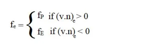
`(v.n)_e` is the velocity component at point e in x direction

Advantages: This scheme satisfies the boundedness criterion, in the sense that irrespective of what the velocity values are and irrespective of what is the grid spacing the solution will always remain bounded

Disadvantages:- 

1. This scheme is numerically diffusive
2. Peak or the rapid variations in the variables will be smeared out
3. Only first order accurate. Very fine grids are required to obtain accurate solutions.

2. Linear Interpolation Scheme:-

It is the simplest and most widely used interpolation. in this case we approximate the values of the variable at Control Volume face centre by interpolating the values linearly at the two nearest computational nodes.

The linear interpolation is equivalent to the use of the central difference formula of the first order derivative and hence it is also called as Central Difference Schemes(CDS). it is second order accurate whose accuracy is very good but we might have one small problem foe advection dominated situations, that this scheme may produce oscillatory solutions, This scheme leads to simple approximation for evaluation of gradients required for evaluation of diffusive fluxes.

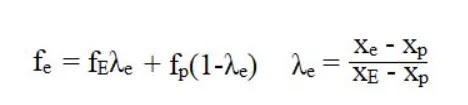
`lambdae`----> Function which would depend on the relative locations of the computational nodes E and P with respect to eastern face.

3. Quadratic upwind interpolation:-

In this case we have to approximate the value of the variable at Control Volume face centre by quadratic interpolation of the values at three nearest computational nodes.(one Downstream node D and 2 upstream nodes U and UU).

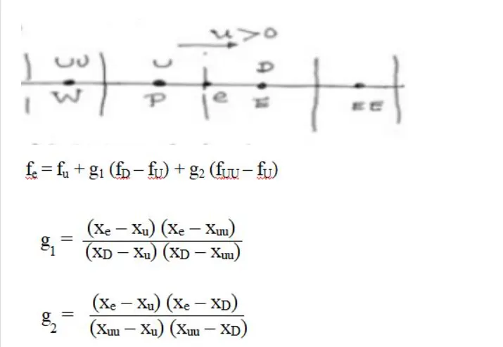
4.Hybrid Scheme:-

This scheme is the combination of Upwind interpolation scheme and Central Distribution seheme based on the loacal Peclet number

`f_e = gamma^fCDS+(1-gamma)f_(CDS)`

5. Total Variation Diminsh:-

`f_e = f_p+0.5*psi*r*(f_e-f_p)`

`psi`-----> Local flux limiter     r------> Specified function which depends upon the local conditions

FLUX LIMITER:-

They are used in high resolution schemes, to avoid the false oscillations that would otherwise occur with high order spatial discretization schemes due to shocks, discontinuties or sharp changes in the solution domain. use of flux limiters, together with an apprpriate high resolution scheme, make the solutions Total Variation Diminishing (TVD). The main idea behind the construction of flux limiters schemes is to limit the spatial derivaties to realistic values The main purpose of flux limiter is to keep the values bounded at the cell faces. Flux limiter don't let the solution value to overshoot.

Consider a 1D semi Discrete scheme

     

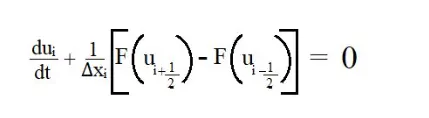
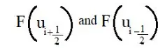
  represents the edge fluxes for the `i^(th)` cell can be represented by low and high resolution schemes then the flux limiter can switch between these schemes depending upon the gradients close to the particular cell.

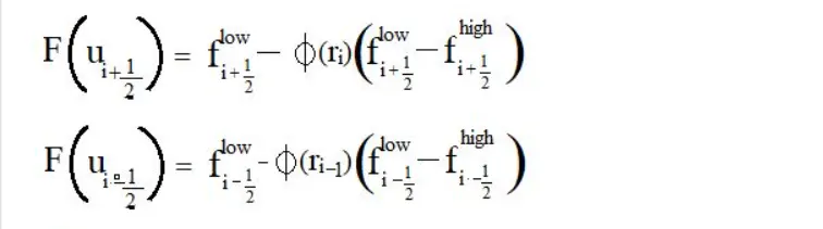
where,

`f^(low)` = Low resolution flux,

`f^(high)` = High resolution flux,

`phi(r)` = flux limiter function,

and r represents the ratio of successive gradients on the resolution mesh, i.e.,

`r_i = (u_i-u_(i-1))/(u_(i+1)-u_i)`