Week 3.5 - Deriving 4th order approximation of a 2nd order derivative using Taylor Table method

Deriving Fourth oredr Approximation of a Second order Derivative using Taylors Table Method

objective:-

To write and execute a MATLAB program for fourth order approximations of the second order derivaties using Taylor,s table method of the funtion exp(x)*cos(x) and compare the results with central difference approcimation and skewed schmes.

INTRODUCTION:-

In this demostration we will evaluvate the 4th order approximation of diffrent schmes for 2nd order derivativs of the function exp(x)*cos(x) and

• plot that will compare the absolute errors between the schmes
• comparasion of the errors with FDS and BDS approximations
• To conclude, how skewed schemes are useful and benifit of it than central scheme
• MATLAB codes with required functions

1. Formulation of the taylor Table methods for CDS

`f''(x) = (af(x-2h)+bf(x-h)+cf(x)+df(x+h)+ef(x+2h))/h^2`

2. Formulation for the taylor table method of Right skewed schme

`f''(x) = (af(x)+bf(x+h)+cf(x+2h)+df(x+3h)+ef(x+4h)+bf(x+5h))/h^2`

3.Formulation for the taylor table method of Left skewed schme

`f''(x) = (af(x)+bf(x-h)+cf(x-2h)+df(x-3h)+ef(x-4h)+bf(x-5h))/h^2`

4.Forward diffrence schme

`f''(x)=( af(x)+bf(x+h)+cf(x+2h))/h^2`

5.backward diffrence schme

`f''(x) =( af(x)+bf(x-h)+cf(x-2h))/h^2`

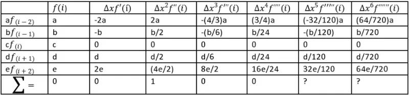
Fourth order centered scheme

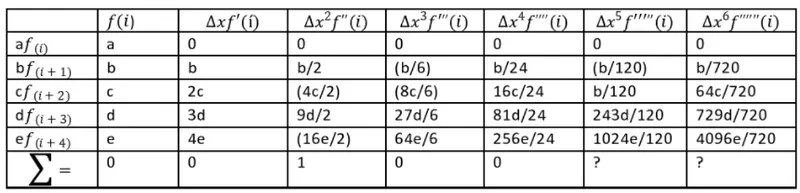
Fourth order Right skewed scheme

Fourth order Left skewed scheme

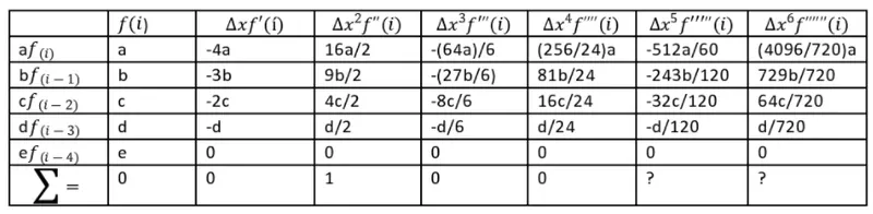
The taylors's table is made by expanding the well known taylor's series. in above equations we need to find the coefficients a,b,c,d and e for each schemes by comparing the coefficents of taylor's series expansion to LHS. To make our life little easier, i have inserted the MATLAB program for execution of these coefficients.

when solving by x=AB, we get the following results for diffrent schemes

1.Fourth order CDS

a=2.91667 b=8.6667 c=9.5 d=8.6667 e=-0.8333

2.Fourth order Right sided skewed scheme

a=2.91667 b=-8.6667 c=9.5 d= -4.6667 e= 0.91667

3.Fourth order Left sided skewed scheme

a=0.91667 b=-4.6667 c=9.5 d=-8.6667 e=2.9167

Note:- The values of approximations wii solely depends on the step size we choose.

Matlab code:-

Function code

1.Fourth order CDS

% Function for 4th order Central Difference scheme
function err_CD = Function_CD2(x,dx)
% Analytical function = exp(x)*cos(x)
% f''(x) = -2*sin(x)*exp(x);
analytical_derivative = -2*sin(x)*exp(x);
% Numerical derivative
CD = ((-0.0833*cos(x-2*dx)*exp(x-2*dx))+(1.3333*cos(x-dx)*exp(x-dx))+(-2.5*cos(x)*exp(x))+(1.3333*cos(x+dx)*exp(x+dx))+(-0.0833*cos(x+2*dx)*exp(x+2*dx)))/dx^2;
err_CD = abs(analytical_derivative - CD);
end

2.Fourth order Right sided skewed scheme

% Function for 4th order Right skewed Difference scheme
function err_SR = Function_RSD5(x,dx)
% Analytical function = exp(x)*cos(x)
% f''(x) = -2*sin(x)*exp(x);
analytical_derivative = -2*sin(x)*exp(x);
% Numerical derivative
SR = ((2.9167*cos(x)*exp(x))+(-8.667*cos(x+dx)*exp(x+dx))+(9.5*cos(x+2*dx)*exp(x+2*dx))+(-4.667*cos(x+3*dx)*exp(x+3*dx))+(0.9167*cos(x+4*dx)*exp(x+4*dx)))/dx^2;
err_SR = abs(analytical_derivative - SR);
end

3.Fourth order Left sided skewed scheme

% Function for 4th order Left skewed Difference scheme
function err_SL = Function_LSD4(x,dx)
% Analytical function = exp(x)*cos(x)
% f''(x) = -2*sin(x)*exp(x);
analytical_derivative = -2*sin(x)*exp(x);
% Numerical derivative
SL = ((0.91667*cos(x)*exp(x))+(-4.667*cos(x-dx)*exp(x-dx))+(9.5*cos(x-2*dx)*exp(x-2*dx))+(-8.667*cos(x-3*dx)*exp(x-3*dx))+(2.9167*cos(x-4*dx)*exp(x-4*dx)))/dx^2;
err_SL = abs(analytical_derivative - SL);
end

4.Function for second order Forward Difference

% Function for Secon order Forward Difference
function err_SO_Forward = Function_FDS3(x,dx)
% Analytical function = exp(x)*cos(x)
% f''(x) = -2*sin(x)*exp(x);
analytical_derivative = -2*sin(x)*exp(x);
% Numerical derivative
SO_Forward = ((exp(x+2*dx)*cos(x+2*dx))+(-2*exp(x+dx)*cos(x+dx))+(exp(x)*cos(x)))/dx^2;
err_SO_Forward = abs(analytical_derivative - SO_Forward );
end

4.Function for second order Backward Difference

% Function for Secon order Backward Difference
function err_SOB = Function_BDS1(x,dx)
% Analytical function = exp(x)*cos(x)
% f''(x) = -2*sin(x)*exp(x);
analytical_derivative = -2*sin(x)*exp(x);
% Numerical derivative
SOB = ((exp(x-2*dx)*cos(x-2*dx))+(-2*exp(x-dx)*cos(x-dx))+(exp(x)*cos(x)))/dx^2;
err_SOB = abs(analytical_derivative - SOB);
end

Main code:-

clear all
close all
clc
x = pi/3;
dx = linspace(0.01,1,15);

for i=1:length(dx)
    err_SO_Forward(i) = Function_FDS3(x,dx(i));
    err_SOB(i) = Function_BDS1(x,dx(i));
    err_CD(i) = Function_CD2(x,dx(i));
    err_SR(i) = Function_RSD5(x,dx(i));
    err_SL(i) = Function_LSD4 (x,dx(i));
    
end 
% To create a plot for using log scale
loglog(dx,err_CD,'r',dx,err_SR,'b',dx,err_SL,'k',dx,err_SO_Forward,'m',dx,err_SOB,'g');
title('Fourth order approximation');
grid on
xlabel('step size"dx"')
ylabel('Errors "dx"')
legend('Central','Right','Left','FDS','BDS')

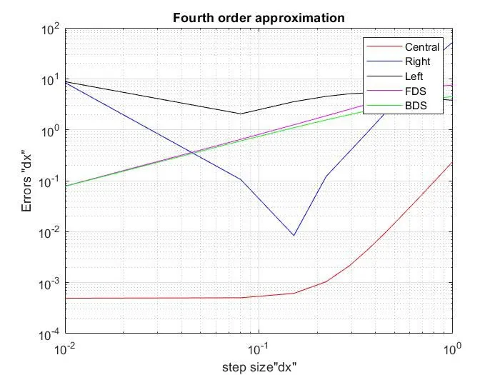
Result of PLOT:-

Result and Discussion:-

As seen on the above plot, the central differencing scheme has very less error compared to other schemes, obiviously it gathers informations from both neighbouring nodes. the FDS and BDS are for 1st oredr approimations of 1st derivative but Fourth -order centred and skewed are for fourth order approximation for second derivatives.

Why Skewed schemes are useful?

When we dont have any nodes at the boundary then skewed schemes are useful to approximate to improve the accuracy but when we have internal nodes available then Centered ones are good though.