Week 5.1 - Mid term project - Solving the steady and unsteady 2D heat conduction problem

Solving Steady and unsteady state 2D Heat Conduction problems

OBJECTIVE:-

To solve Steady and unsteady state 2D Heat Conduction Equation by using the point iterative techniques such as jacobi, Gauss seidel & Successive over relaxationfor both implicit and explicit schemes using MATLAB.

Problem statement:-

• Computation area is to be a square.
• Assume nx = ny[No. of points x-direction is equal to no. of points in y-direction]
• We assume nx=ny=10
• Boundary conditions are

Left = 400k

Right = 600k

Top = 800k

Bottom = 900k

• Apart from the boundary conditions, all other nodes are given an initial temprature of 300k.
• Various methods to be employed in solving the equation are given below.

1. Various states:- Steady-state & unstedy-state Condition
2. Various schmes:- jacobi, Gauss-seidel & Successive over-relaxation
3. Various Methods to be used in Unstedy-state:- Implicit & Explicit

By using point iterative method, solve the 2D Heat conduction equation and plot the temprature contour for all the three iterative methods namely jacobi,Gauss-Seidel & SOR for steady and unsteady conditions under IMPLICIT scheme also additionally solving the EXPLICIT scheme for Unsteady condition.

THEORY:-

The heat equation is a partial diffrential equation that describes how the distribution of some quantity (such as heat) evolves over time in a solid medium, as it spontaneously flows from places where it higher towards places where it lower.

For function u(x,y,z,t) of three spatial variables (x,y,z) (see Cartesian coordinate system) and the time variablet. the heat

`(partialu)/(partialt)=alpha((partial^2u)/(partialx^2)+(partial^2u)/(partialy^2)+(partial^2u)/(partialz^2))`

where,

`alpha` is areal coefficient called the diffusivity of the medium.

Types of Heat Conduction schemes

This transfer of Heat energy may occur under two conditions

• Steady-state condition
• Unsteady/Transient state condition

Unsteady state conditions are a precursor to steady state conditions. No system exists initially under steady state conditions. Some time must pass, after heat transfer is initiated, before the system reaches steady state. During the period of transition the systemis under unsteady state conditions.

Time Loop Logic:-

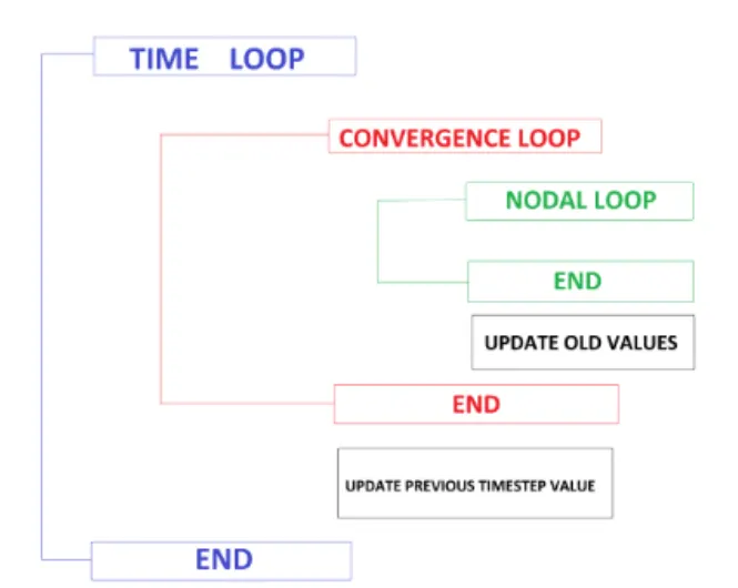
Boundary Condition:-

T_L =Left boundary

T_T = Top boundary

T_R = Right boundary

T_B =Bottom boundary

Governing Equations:-

In order to solve the 2D Heat conduction problem, the governing equations for resoective conditions with respect to cartesian coordinates should be discretized to enter that in a code which is given under MAIN PROGRAM below.

MAIN PROGRAM:-

Below there is a sequence of seven invidividual programs, starting with IMPLICIT Scheme of Steady & unsteady-state conditions for three iterative methods jacobi,gauss-seidel & SOR followed by EXPLICIT scheme for Unsteay/Transient conditions.

IMPLICIT Scheme-Steady-state Condition Program:-

In steady-state conduction, the amount of heat entering any region of an object is equal to the amount of heat coming out (if this were not so, the temprature would be rising or falling, as thermal energy was tapped or trapped in a region).

`(partial^2T)/(partialx^2)+(partial^2T)/(partialy^2)=0`

By discretizing the equation above it becomes,

`T_p =(1/k)[(T_L+T_r)/(trianglex^2)+(T_T+T_B)/(triangley^2)]`

Here the vaklue of k is

`K =2((trianglex^2+triangley^2)/(trianglex^2triangley^2))`

if we further simply this the equation for code becomes

`0.25.(T_L+T_R+T_T+T_B)`

which can also be written as,

`T_i,_j = 0.25(T_(i-1),_j+T_(i+1),_j)+T_(i,(j-1)+T_(i,(j+1)))`

Jacobi Iteration:-

% Solving the stedy state 2D Heat conduction  (jacobi method)
clear all
close all
clc
% Input Parameters
%Number of grid points
nx = 10;
ny = 10;
x = linspace(0,1,nx);
y = linspace(0,1,ny);
dx = x(2) - x(1);
dy = dx;
% Absolute error criteria > tolerance
error = 9e9;
tolerance = 1e-4;
% Defining Boundary Conditions
T_L = 400;
T_T = 600;
T_R = 800;
T_B = 900;
T = 300*ones(nx,ny);
T(2:ny - 1,1) = T_L;
T(2:ny - 1,nx) = T_R;
T(1, 2:nx - 1) = T_T;
T(ny, 2:nx -1) = T_B;
% Calculating Average temprature at corners
T(1,1) = (T_T + T_L)/2;
T(nx,ny) = (T_R + T_B)/2;
T(1,ny) = (T_T + T_R)/2;
T(nx,1) = (T_L + T_B)/2;
% Assigning original value to T
T_initial = T;
T_old = T;
% Calculation of 2D Heat Conduction Equation by Jacobi method
iterative_solver = 1;
if iterative_solver == 1
    jacobi_iteration = 1;
    
    while(error > tolerance)
        for i = 2:nx -1
            for j = 2:ny - 1
                T(i,j) = 0.25*(T_old(i-1,j)+ T_old(i+1,j)+T_old(i,j-1)+T_old(i,j+1));
            end
        end
        error = max(max(abs(T_old - T)));
        T_old = T;
        jacobi_iteration = jacobi_iteration + 1;
    end
end
% Plotting
figure(1)
contour(x,y,T)
clabel(contourf(x,y,T))
colorbar
colormap(jet)
set(gca,'ydir','reverse')
xlabel('x-axis')
ylabel('y-axis')
title(sprintf('No. of jacobi Iterations (Implicit) = %d',jacobi_iteration));
pause(0.03);

OUTPUT:-

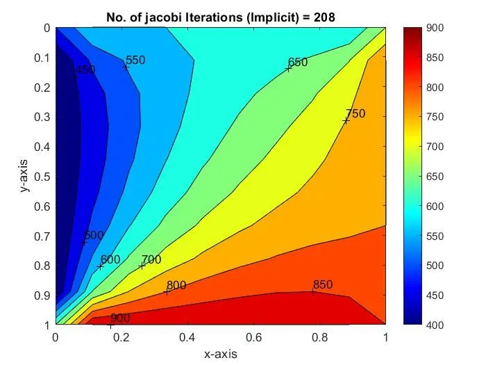
Gauss-Seidel Iteration:-

% Solving the stedy state 2D Heat conduction  (Gauss-seidalmethod)
clear all
close all
clc
% Input Parameters
%Number of grid points
nx = 10;
ny = 10;
x = linspace(0,1,nx);
y = linspace(0,1,ny);
dx = x(2) - x(1);
dy = dx;
% Absolute error criteria > tolerance
error = 9e9;
tolerance = 1e-4;
% Defining Boundary Conditions
T_L = 400;
T_T = 600;
T_R = 800;
T_B = 900;
T = 300*ones(nx,ny);
T(2:ny - 1,1) = T_L;
T(2:ny - 1,nx) = T_R;
T(1, 2:nx - 1) = T_T;
T(ny, 2:nx -1) = T_B;
% Calculating Average temprature at corners
T(1,1) = (T_T + T_L)/2;
T(nx,ny) = (T_R + T_B)/2;
T(1,ny) = (T_T + T_R)/2;
T(nx,1) = (T_L + T_B)/2;
% Assigning original value to T
T_initial = T;
T_old = T;
% Calculation of 2D Heat Conduction Equation by Gauss - seidel method
iterative_solver = 2;
if iterative_solver == 2
    Gauss_seidel_iteration = 1;
    
    while(error > tolerance)
        for i = 2:nx -1
            for j = 2:ny - 1
                T(i,j) = 0.25*(T(i-1,j)+ T_old(i+1,j)+T(i,j-1)+T_old(i,j+1));
            end
        end
        error = max(max(abs(T_old - T)));
        T_old = T;
       Gauss_seidel_iteration = Gauss_seidel_iteration + 1;
    end
end
% Plotting
figure(2)
contour(x,y,T)
clabel(contourf(x,y,T))
colorbar
colormap(jet)
set(gca,'ydir','reverse')
xlabel('x-axis')
ylabel('y-axis')
title(sprintf('No. of Gauss-seidel Iterations (Implicit) = %d',Gauss_seidel_iteration));
pause(0.03);

Output:-

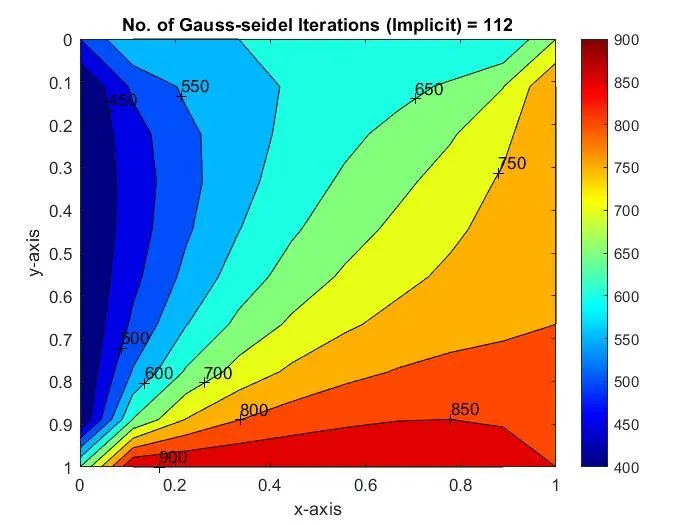
SOR Method:-

% Solving the stedy state 2D Heat conduction  (Successive Over relaxation method)
clear all
close all
clc
% Input Parameters
%Number of grid points
nx = 10;
ny = 10;
x = linspace(0,1,nx);
y = linspace(0,1,ny);
dx = x(2) - x(1);
dy = dx;
% Absolute error criteria > tolerance
error = 9e9;
tolerance = 1e-4;
omega = 1.2;
% Defining Boundary Conditions
T_L = 400;
T_T = 600;
T_R = 800;
T_B = 900;
T = 300*ones(nx,ny);
T(2:ny - 1,1) = T_L;
T(2:ny - 1,nx) = T_R;
T(1, 2:nx - 1) = T_T;
T(ny, 2:nx -1) = T_B;
% Calculating Average temprature at corners
T(1,1) = (T_T + T_L)/2;
T(nx,ny) = (T_R + T_B)/2;
T(1,ny) = (T_T + T_R)/2;
T(nx,1) = (T_L + T_B)/2;
% Assigning original value to T
T_initial = T;
T_old = T;
% Calculation of 2D Heat Conduction Equation by Gauss - seidel method
iterative_solver = 3;
if iterative_solver == 3
    Successive_Over_Relaxation_iteration = 1;
    
    while(error > tolerance)
        for i = 2:nx -1
            for j = 2:ny - 1
                T(i,j) = omega*(0.25*(T(i-1,j)+ T_old(i+1,j)+T(i,j-1)+T_old(i,j+1)))+ (1 - omega)*T_old(i,j);
            end
        end
        error = max(max(abs(T_old - T)));
        T_old = T;
      Successive_Over_Relaxation_iteration = Successive_Over_Relaxation_iteration + 1;
    end
end
% Plotting
figure(3)
contour(x,y,T)
clabel(contourf(x,y,T))
colorbar
colormap(jet)
set(gca,'ydir','reverse')
xlabel('x-axis')
ylabel('y-axis')
title(sprintf('No. of Successive-Over Relaxation iterations(Implicit) = %d',Successive_Over_Relaxation_iteration));
pause(0.03);

Output:-

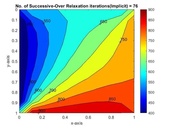
IMPLICIT scheme Unsteady/Transient-state Condition:-

Unsteady-state Equation Discretization:-

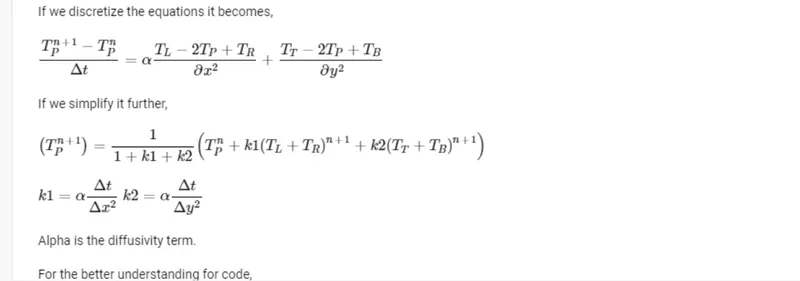
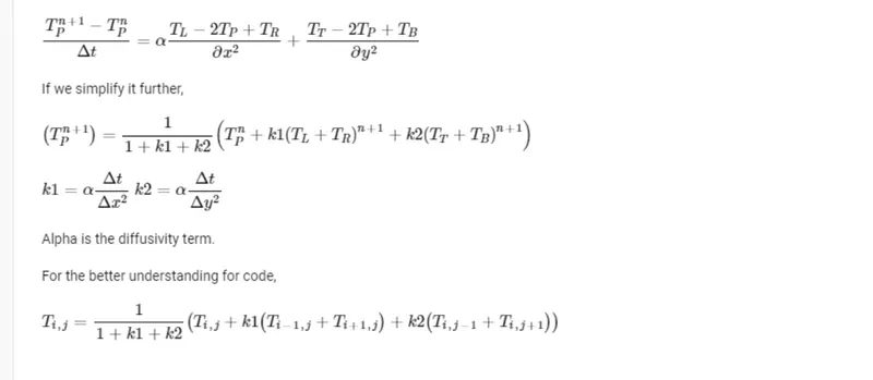
Non-steady-state situations appear after an imposed change in temprature at a boundary as well as inside of an object, as a result of a new source or sink of heat suddenly introduced within object, causing tempratures near the source or sink to change in time.

`(partialT)/(partialt)=alpha(partial^2T)/(partialx^2)+(partial^2T)/(partialy^2)`

Jacobi Iteration:-

% Solving the Unstedy state 2D Heat conduction (Jacobi method)(Implicit)
clear all
close all
clc
% Input Parameters 
% Number of grid points
nx = 10;
ny = nx;
nt = 1400;
x = linspace(0,1,nx);
y = linspace(0,1,ny);
dx = x(2) - x(1);
dy = dx;
% Absolute error criteria > tolerance
error = 9e9;
tolerance = 1e-4;
dt = 1e-3;

% Defining Boundary condition
T_L = 400;
T_T = 600;
T_R = 800;
T_B = 900;
T = 300*ones(nx,ny);
T(2:ny - 1,1) = T_L;
T(2:ny - 1,nx) = T_R;
T(1, 2:nx - 1) = T_T;
T(ny, 2:nx -1) = T_B;
% Calculating Average temprature at corners
T(1,1) = (T_T + T_L)/2;
T(nx,ny) = (T_R + T_B)/2;
T(1,ny) = (T_T + T_R)/2;
T(nx,1) = (T_L + T_B)/2;
% Assigning original value to T
T_old = T;
T_intial = T;
% Calculation of 2D stedy state conduction equation by Jacobi method
k1 = 1.1*(dt/(dx^2));
k2 = 1.1*(dt/(dy^2));
jacobi_iteration = 1;
for k = 1:nt
    error = 9e9;
    while(error > tolerance)
        for i = 2:nx - 1
            for j = 2:ny - 1
                Term_1 = 1/(1+ (2*k1)+ (2*k2));
                Term_2 = k1*Term_1;
                Term_3 = k2*Term_1;
                H = (T_old(i-1,j)) + (T_old(i+1,j));
                V = (T_old(i,j+1)) + (T_old(i,j-1));
                
                T(i,j) = (T_intial(i,j)*Term_1) + (H*Term_2) + (V*Term_3);
            end
        end
        error =  max(max(abs(T_old-T)));
        T_old = T;
        jacobi_iteration = jacobi_iteration + 1;
    end
    T_intial = T;
    % Plotting 
    figure(1)
    contourf(x,y,T)
    clabel(contourf(x,y,T))
    colorbar
    colormap(jet)
    set(gca,'ydir','reverse')
    xlabel('x-Axis')
    ylabel('y-Axis')
    title(sprintf('No.of unsteady jacobi Iterations (implicit) = %d',jacobi_iteration));
    pause(0.03)
end
        

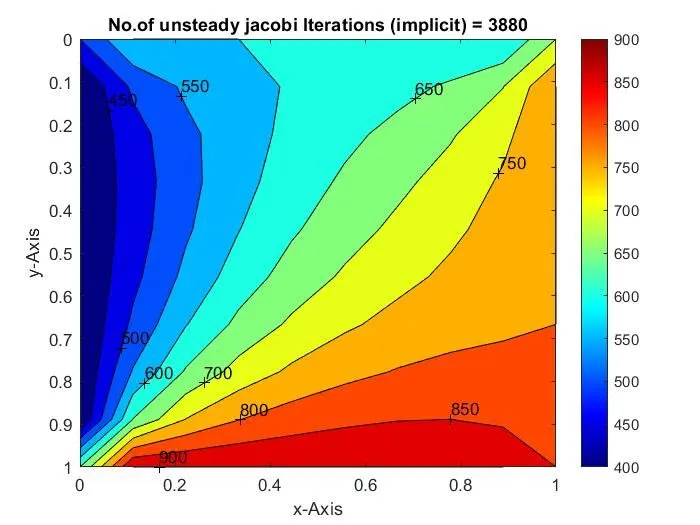
Output:-

Gauss-Seidel Iteration:-

% Solving the Unstedy state 2D Heat conduction (Gauss-seidel method)(Implicit)
clear all
close all
clc
% Input Parameters 
% Number of grid points
nx = 10;
ny = nx;
nt = 1400;
x = linspace(0,1,nx);
y = linspace(0,1,ny);
dx = x(2) - x(1);
dy = dx;
% Absolute error criteria > tolerance
error = 9e9;
tolerance = 1e-4;
dt = 1e-3;

% Defining Boundary condition
T_L = 400;
T_T = 600;
T_R = 800;
T_B = 900;
T = 300*ones(nx,ny);
T(2:ny - 1,1) = T_L;
T(2:ny - 1,nx) = T_R;
T(1, 2:nx - 1) = T_T;
T(ny, 2:nx -1) = T_B;
% Calculating Average temprature at corners
T(1,1) = (T_T + T_L)/2;
T(nx,ny) = (T_R + T_B)/2;
T(1,ny) = (T_T + T_R)/2;
T(nx,1) = (T_L + T_B)/2;
% Assigning original value to T
T_old = T;
T_intial = T;
% Calculation of 2D stedy state conduction equation by Gauss-seidel method
k1 = 1.1*(dt/(dx^2));
k2 = 1.1*(dt/(dy^2));
Gauss_seidel_iteration = 1;
for k = 1:nt
    error = 9e9;
    while(error > tolerance)
        for i = 2:nx - 1
            for j = 2:ny - 1
                Term_1 = 1/(1+ (2*k1)+ (2*k2));
                Term_2 = k1*Term_1;
                Term_3 = k2*Term_1;
                H = (T(i-1,j)) + (T_old(i+1,j));
                V = (T(i,j+1)) + (T_old(i,j-1));
                
                T(i,j) = (T_intial(i,j)*Term_1) + (H*Term_2) + (V*Term_3);
            end
        end
        error =  max(max(abs(T_old-T)));
        T_old = T;
        Gauss_seidel_iteration = Gauss_seidel_iteration + 1;
    end
    T_intial = T;
    % Plotting 
    figure(1)
    contourf(x,y,T)
    clabel(contourf(x,y,T))
    colorbar
    colormap(jet)
    set(gca,'ydir','reverse')
    xlabel('x-Axis')
    ylabel('y-Axis')
    title(sprintf('No.of unsteady Gauss-seidel iterations (implicit) = %d',Gauss_seidel_iteration));
    pause(0.03)
end
        

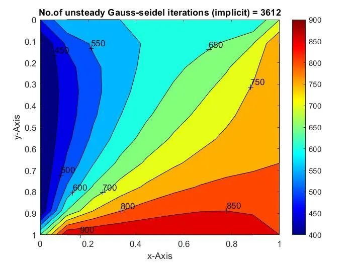
Output:-

SOR Method:-

% Solving the Unstedy state 2D Heat conduction (Successive Over Relaxation  method)(Implicit)
clear all
close all
clc
% Input Parameters 
% Number of grid points
nx = 10;
ny = nx;
nt = 1400;
x = linspace(0,1,nx);
y = linspace(0,1,ny);
dx = x(2) - x(1);
dy = dx;
% Absolute error criteria > tolerance
error = 9e9;
tolerance = 1e-4;
dt = 1e-3;
omega = 1.1;

% Defining Boundary condition
T_L = 400;
T_T = 600;
T_R = 800;
T_B = 900;
T = 300*ones(nx,ny);
T(2:ny - 1,1) = T_L;
T(2:ny - 1,nx) = T_R;
T(1, 2:nx - 1) = T_T;
T(ny, 2:nx -1) = T_B;
% Calculating Average temprature at corners
T(1,1) = (T_T + T_L)/2;
T(nx,ny) = (T_R + T_B)/2;
T(1,ny) = (T_T + T_R)/2;
T(nx,1) = (T_L + T_B)/2;
% Assigning original value to T
T_old = T;
T_intial = T;
T_end = T;
% Calculation of 2D stedy state conduction equation by Successive Over Relaxation method
k1 = 1.1*(dt/(dx^2));
k2 = 1.1*(dt/(dy^2));
Successive_Over_Relaxation_iteration = 1;
for k = 1:nt
    error = 9e9;
    while(error > tolerance)
        for i = 2:nx - 1
            for j = 2:ny - 1
                Term_1 = 1/(1+ (2*k1)+ (2*k2));
                Term_2 = k1*Term_1;
                Term_3 = k2*Term_1;
                H = (T(i-1,j)) + (T_old(i+1,j));
                V = (T(i,j+1)) + (T_old(i,j-1));
                
                T(i,j) = (T_intial(i,j)*Term_1) + (H*Term_2) + (V*Term_3);
                T_end(i,j) = ((1-omega)*T_old(i,j)) + (T(i,j)*omega);
            end
        end
        error =  max(max(abs(T_old-T)));
        T_old = T_end;
        Successive_Over_Relaxation_iteration = Successive_Over_Relaxation_iteration + 1;
    end
    T_intial = T;
    % Plotting 
    figure(1)
    contourf(x,y,T)
    clabel(contourf(x,y,T))
    colorbar
    colormap(jet)
    set(gca,'ydir','reverse')
    xlabel('x-Axis')
    ylabel('y-Axis')
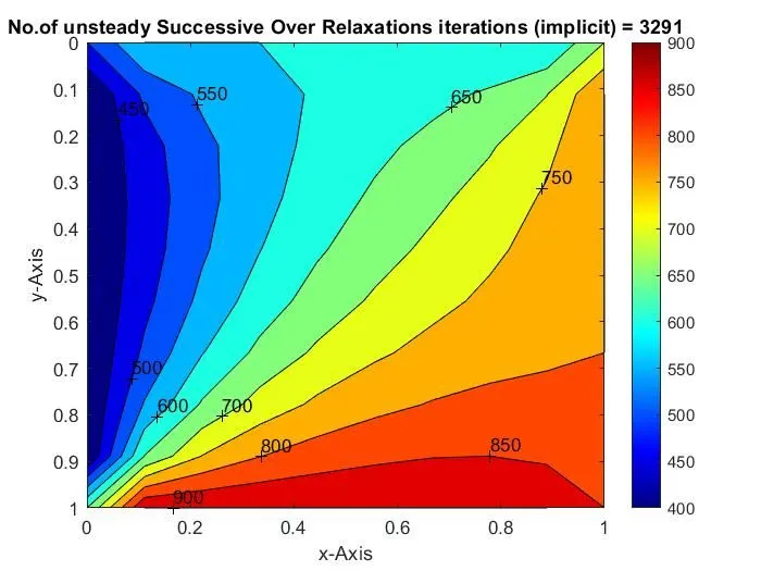
    title(sprintf('No.of unsteady Successive Over Relaxations iterations (implicit) = %d',Successive_Over_Relaxation_iteration));
    pause(0.03)
end
        

Output:-

EXPLICIT SCHEME - Unsteady/Transient State Condition Program:-

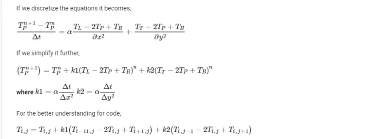
Unsteady-state Equation Discretization[EXPLICIT]:-

`(partialT)/(partialt)=alpha(partial^2T)/(partialx^2)+(partial^2T)/(partialy^2)`

EXPLICIT Scheme:-

T = 300*ones(nx,ny);
T(2:ny - 1,1) = T_L;
T(2:ny - 1,nx) = T_R;
T(1, 2:nx - 1) = T_T;
T(ny, 2:nx -1) = T_B;
% Calculating Average temprature at corners
T(1,1) = (T_T + T_L)/2;
T(nx,ny) = (T_R + T_B)/2;
T(1,ny) = (T_T + T_R)/2;
T(nx,1) = (T_L + T_B)/2;
% Assigning original value to T
T_intial = T;
T_old = T;
% Calculation of 2D stedy state conduction equation by Explicit  method
iterative_solver = 1;
k1 = 1.1*(dt/(dx^2));
k2 = 1.1*(dt/(dy^2));
  if iterative_solver == 1
    Steady_Explicit = 1;
for k = 1:nt
    error = 1;
    while(error > tolerance)
        for i = 2:nx - 1
            for j = 2:ny - 1
                Term_1 = T_old(i,j);
                Term_2 = k1*(T_old(i+1,j) - 2*T_old(i,j) + (T_old(i-1,j)));
                Term_3 = k2*(T_old(i,j+1) - 2*T_old(i,j) + (T_old(i,j-1)));
                T(i,j) = Term_1 +Term_2 +Term_3;
            end
        end
        error =  max(max(abs(T_old-T)));
        T_old = T;
         Steady_Explicit = Steady_Explicit+ 1;
    end
end
end

    T_intial = T;
    % Plotting 
    figure(1)
    contourf(x,y,T)
    clabel(contourf(x,y,T))
    colorbar
    colormap(jet)
    set(gca,'ydir','reverse')
    xlabel('x-Axis')
    ylabel('y-Axis')
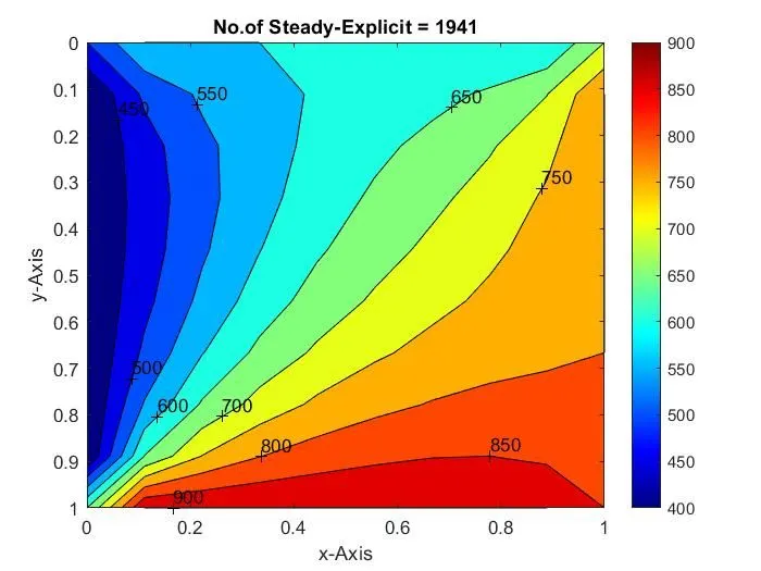
    title(sprintf('No.of Steady-Explicit = %d',Steady_Explicit));
    pause(0.03)

Output:-

CONCLUSIONS:-

Types of Schemes & Analysis	Various methods	No.of Iterations
IMPLICIT-Steady staete Analysis	Jacobi	208
	Gauss_siedel	112
	Successiver Over Relaxation	76
IMPLICIT-Steady staete Analysis	Jacobi	3880
	Gauss_siedel	3612
	Successiver Over Relaxation	3291
EXPLICIT Analysis		1941

From the above outputs of various methods & comparing their No. of iterations we can conclude that

• jacobi> Gauss-seidel> Successive over-Relaxation according to the No.of iterations computed for all methods & schemes.
• When comparing Steady state and Unsteady state, it is proven that Steady state is the most successful one as it takes least number of iterations and least time to compute.
• SOR iteration method is the most effective iteration method as it took at least No. of iterations for coverging solutions in both the schemes (EXPLICIT & IMPLICIT) compared to jacobi & Gauss-sidel.