Week 9 - FVM Literature Review
Objective :
1) Explain what is Finite Volume Method .
2) Explain major difference between FDM and FVM .
3) Explain need for interpolation schemes and flux limiters in FVM .
Answers :
1) In finite volume method , we convert the given differential equation into divergence form. This effectively writes the equations using divergence operators . THe equation is then integrated over entire volume. We then apply Gauss's Theorem to convert the volume integral over the divergence to a surface integral across the boundaries. The integral is therefore turned from integrating the differential of the dependant variable inside of the cells into surface integral of the fluxes of the dependant variable across the boundary of the cells . These integrals are then calculated using suitable numerical approximation methods .
By monitoring the fluxes of the dependant variables across the boundary of the cells ,a conservation approach of the dependant variable is obtained. This is in contrast to FDM , which seeks to approximate the differentials of the differential equation i.e the changes of the dependant variable across the cell .
Example
Let us consider 1D steady state heat equation .
`del /(delx)(alpha.(delT)/(delx))+ S =0`
Where S is the source term responsible for heat generation .
In finite volume method , our geometry is divide into number of control volume called cells. Each cell has a node in its centre where the properties are calculated .
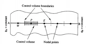
Let us consider 3 cells with central nodes W, P , E and cennecting faces w,e .
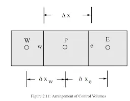
Applying the above equation ,
`int (del/(delx)(alpha.(delT)/(delx))+S)dV =0`
Applying Gauss divergence theorem and expanding , we have
`intdel/(delx)(alpha.(delt)/(delx))A.dx + intS.dV=0`
where A is the face area
dV= control volume
dx= distance between 2 nodes .
`alpha` = Thermal conductivity
`[alpha.A.(delt)/(delx)]_w^e + barS.dV=0`
where `barS` = is the average value of S which satisfies condition `barS.dV=intS.dV`
`alpha_e.A.(delT)/(delx_e) - alpha_w.A.(delT)/(delx_w)+barS.dV=0`
`alpha.A.[T_E-T_P]/(trianglex) - alpha.A.[T_P-T_W]/(trianglex)+barS.dV=0`
The first term is heat flux in . the second term is heat flux out . This is how conservation is maintained .
2)
Major difference between FVM and FDM are as follows .
a) Finite Difference method or FDM is mostly used for defined geometries which could be represented by structured grids whereas FVM calculates properties for every cell(controlled volumes)hence can be used for complicated geometries .
b) FDM uses differential form of governing equations whereas FVM uses integral fom of governing equations .
c) It is easy to increase the element order in-order to get higher order accuracy in case if FDM. In FVM it is not easy to increase the accuracy by increasing the functions to higher order
d) In FDM , it is not possible to do local grid refinement or adaptive mesh refinement . In FVM, we can increase local accuracy by refining mesh in those areas .
e) By monitoring the fluxes of the dependant variables across the boundary of the cells, a conservation approach of the dependant variable is obtained in case of FVM . This is in contrast to FDm, which seeks to approximate the differentials of the differential equation i.e the changes of the dependant variable across each cell .
3)
a) Interpolation in FVM
The approximation of surface and volume intergrals may require values of the variable at locations other than the computational nodes of the controlled volume . Values at these locations are obtained using interpolation formulae .
There are 3 main types of interpolation used in FVM .
i) Upwind Interpolation
The upwind interpolation scheme (UDS) for approximating thevalue of a variable of the east face of a control volume is given by
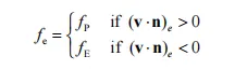
This interpolation scheme is equivalent to using a backward or forward finite difference approximation (depending on the flow direction). It is first order accurate , and is numerically diffussive with co-efficient of diffussion
`eta_e^n = (rhou)_e.(trianglex)/2`
ii) Linear Interpolation (CDS)
We can approximate the value of the variable at controlled volume face by linear interpolation of the values at two nearest computational nodes . Thus , at location 'e' on a cartesian grid , the variable value is approximated by
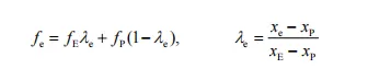
The linear interpolation is equivalent to use of central differencing formula of the first order derivative and hence, this scheme is also termed as central differencing scheme (CDS). This scheme is second order accurate and may produce oscillatory solutions .
iii) Quadratic upwind Interpolation (QUICK)
A quadratic upwind interpolation scheme can be derived using polynomial fitting . The QUICK interpolation on a uniform cartesian grid i sgiven by
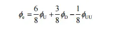
where D , U and UU denote the down stream , the first upstream and 2nd upstream node respectively . (E,P and W or P, E or EE depending on the flow direction ) . QUICK scheme is third order accurate but prone to oscillations .
b)
Total Variation Diminishing
Total variation diminishing is the property of a solution by which the total variation in a discrete solution reduces by time . Total variation is considered at every time step and a solution is said to be TVD if
`TV(phi^(n+1)) <= TV (phi^n)`
where n and n+1 refer to the consecutive time steps .
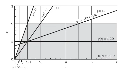
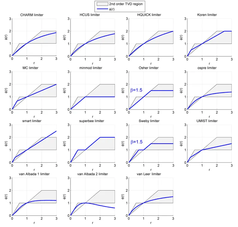
The shaded region in the above diagram shows the shaded region in which solutions under various interpolation schemes have TVD property .
Flux limiter functions
The Idea of designing is to introduce a modification to the above schemes so as to force the `r-psi` relationship to remain within the shaded region for all possible values of r . This implies that , in order to make a scheme TVD , we must constrain or limit the range of possible values of the additional convective flux `F_e psi(r)(phi_E-phi_p)/2`, which was originally introduced to make the scheme higher order . Hence the function `psi(r)` is called flux limiter function.
Given below are a list of popular flux limiter functions .
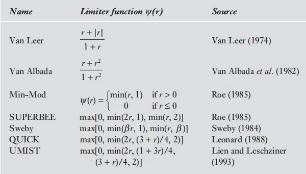
Given below is an image of plots for various types of fluz limiter functions .