Week 9 - FVM Literature Review

STUDY ON FVM

FINITE VOLUME METHOD (FVM):

The Finite Volume Method (FVM) is one of the most versatile discretization techniques used in CFD. The most interesting feature of the FVM is that the resulting solution satisfies the conservation of mass, momentum and energy. This is exactly satisfied for any control volume as well as for the whole computational domain and for any number of control volumes.

FVM is the ideal method for solving discontinuous problems arising in compressible flows. Any discontinuity must satisfy the Rankine-Hugoniot jump condition, which is a consequence of conservation. Since finite volume methods are conservative, they automatically satisfy the jump conditions and hence give physically correct weak solutions.

MAJOR DIFFERENCE BETWEEN FDM AND FVM:

Finite Difference Method (FDM)	Finite Volume Method (FVM)
1. In Finite difference method, discretization is based on the “differential form” of the Governing Equations to be solved.	1. In Finite volume method, discretization is based on the “integral form” of the Governing Equations to be solved.
2. The computational domain is usually divided into hexahedral cells (the grid), and the solution will be obtained at each nodal point.	2. The computational domain is discretized into finite volumes and then for every volume the governing equations are solved.
3. The discretization results in a system of equation of the variable at nodal points, and once a solution is found, then we have a discrete representation of the solution.	3. The discretization results in a system of equation of the variable at cell center and if the nodal or face values are required, it can be obtained by Interpolation Scheme.
4. The discretized equations are not necessarily conservative in nature for every case in FDM.	4. The discretization equation expresses the conservation principle for the variables inside the control volume, and for any number of control volumes within the computational domain.

INTERPOLATION SCHEMES:

In FVM, we use he integral form of the Governing equation to solve a problem. While doing so, we might need some other additional information as well from points other than the cell centroid like the face center or boundary or so on. To do so, we need a technique or formulae to get the information at the necessary points, and this technique is called as the interpolation technique or scheme.

Consider an example of 1D heat conduction through a fin with a heat source S, the governing equation is;

` del/(delx)(alpha(delT)/(delx))+S=0`

Where, `alpha` is thermal diffusivity which depends on the Temperature at a given point, so it is also a function of ‘T'.

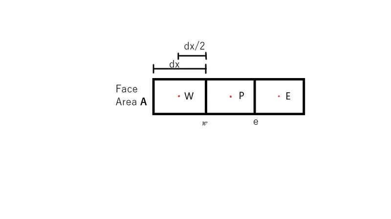
In this figure, we consider P, W and E as the cell centers of the respective cells. To calculate the temperature at the point P, we take information from the neighboring cells W and E so this is called as “Gradient Scheme”. The above governing equation is not only valid for that point but for the whole Control Volume, so,

`int(del/(delx)(alpha(delT)/(delx))+ S)dV=0`

`int(del/(delx)(alpha(delT)/(delx)))dV+ intSdV=0`

Since the small volume dV is equal to face area A multiplied with dx,

`int(del/(delx)(alpha(delT)/(delx)))Adx+ intSdV=0`

The lower and upper limits of integration are ‘w’ and ‘e’ respectively, so, after applying the limits of integration, we get,

`alphaA((delT)/(delx))_E-alphaA((delT)/(delx))_W+ barSdV=0`

`alphaA((T_E-T_P)/(dx))-alphaA((T_P-T_W)/(dx))+ barSdV=0`

By applying forward and backward differencing for east and west sides, we arrived at the above equation.

The above equation shows that the FVM works on conservation of flux. Here, it is ;

Heat flux Out – Heat flux In + Source = 0

Also, we know that `alpha` is a function of T, so the above equation is like;

`alpha_eA((T_E-T_P)/(dx))-alpha_wA((T_P-T_W)/(dx))+ barSdV=0`

So, we need the values of `alpha_e` and `alpha_w`, for which we need the values of `T_e` and `T_w` which are unknown. To get the values, we use the “Interpolation Scheme”.

There are several types of Interpolation schemes, namely;

• Upwind Interpolation Scheme (UDS)
• Linear Interpolation Scheme or Central Differencing Scheme (CDS)
• Quadratic Upwind Interpolation Scheme (QUICK)

FLUX LIMITERS:

Flux limiters are kind of like dampers used in regions where the shocks, discontinuities or sharp change occurs in the solution domain. Basically, they damp the divergence of solution to avoid vigorous oscillations due to shocks by limiting the spatial derivatives to a more realistic value. These flux limiters operate only in the presence of sharp wave fronts, and for smoothly changing waves, the flux limiters do not operate and the spatial derivatives can be represented by higher order approximations without introducing spurious oscillations. There are various limiters which are chosen according to the engineering CFD problem with solution scheme and no limiter is found to work well for all the problems. The Flux Limiter Function, `phi(r)` is constrained to be greater than or equal to zero, i.e., `phi>=0`. So, when the limiter is equal to zero (sharp gradient, opposite slopes or zero gradient), the flux is represented by a low-resolution scheme. Similarly, when the limiter is equal to 1 (smooth solution), it is represented by a high-resolution scheme. Some examples of Flux Limiter Functions are;

• CHARM
• HCUS
• HQUICK
• Koren and so on.

RESULTS:

Thus the study on FVM in the application of CFD is done successfully.