Week 3 - Solving second order ODEs

STUDY ON THE 2nd ORDER ODE USING
A SIMPLE PENDULUM

AIM:
To study the 2nd order Ordinary Differential Equation (ODE) using a simple pendulum experiment on Matlab software.

OBJECTIVES:
⦁ To determine the angular velocity and angular displacement with respect to time of a simple pendulum.
⦁ To plot the graph for various values of angular velocities and angular displacements with respect to time.
⦁ To track and make a movie of the motion of this simple pendulum.

GOVERNING EQUATIONS:
1. The ODE for motion of a simple pendulum with damping is;

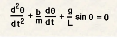
where, 'b' is damping coefficient
'g' is acceleration due to gravity (m/s^2)
'l' is the length of string (m)
'm' is mass of ball (kg)

2. Runge-Kutta method to solve 1st order ODE are;
For this method, we need,
(i) Initial conditions (t_0,y_0)
(ii) Step size, h


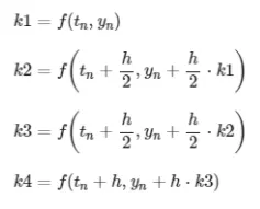
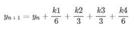
So, y_1 can be calculated and with (t_1,y_1), we can calculate y_2 and so on upto required y_n values.

PROCEDURE:
⦁ This whole program for solving 2nd order ODE of a simple pendulum is coded using Matlab software.
⦁ For this program, we need to solve the 2nd order ODE by discritizing into two 1st order ODEs to get the required 'Angular velocity' and 'Angular displacement' parameters.
⦁ So after splitting the 2nd order ODE, we get two 1st order ODEs, namely;
,

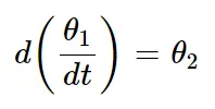where, θ = θ1;
implies, dθ/dt = dθ1/dt = θ2
⦁ Therefore, by integration the above equations, we get the values for θ1 (Angular displacement) and θ2 (Angular velocity) values corresponding to differnt values of time.

% Program to solve 2nd order ODE for a simple pendulum
% ode45 solver is used which uses Runge-Kutta equation for solution
% so we need initial conditions and step size
clear all;
close all;
clc;

% Initial condition;
theta_0 = [0 ; 3];

% Step size values
t_span = linspace(0,20,700);

% Input values
b = 0.05;% damping coefficient
g = 9.81;% acceleration due to gravity (m/s^2)
l = 1;% length of pendulum (m)
m = 1;% mass of pendulum (kg)
n = 1;% counter used to get frames for movie

% ode45 command is an ODE solver which makes use of RK method for solution
% Solving ode in a separate function
[t, results] = ode45(@(t, theta) ode_function(t,theta,b,g,l,m),t_span,theta_0);

% Plotting the results figure for angular velocity and angular displacement
% with respect to time
figure(1);
hold on;
plot(t, results(:,1),'Displayname','Angular Displacement (rad)');% results(:,1) implies that all the rows and 1st column of results matrix is selected.
plot(t, results(:,2),'Displayname','Angular Velocity (rad/s)');% results(:,2) implies that all the rows and 2nd column of results matrix is selected.
xlabel('Time (s)');
ylabel('Results');
legend;

% To get the animated movie for angular displacement of the pendulum with
% respect time, we use for loop;
for i = 1:700 % since t_span has 700 values of time
    Theta = results(i,1);% results(i,1) represents the ith row and 1st column of the results matrix
    disp_x = l*sind(Theta);% Theta values are represented in degree because we just need the coordinates for X and Y to plot the line 
    disp_y = -l*cosd(Theta);
    x0 = 0;% since one end of the pendulum is fixed
    y0 = 0;
    
    figure(2);
    plot([x0 disp_x],[y0 disp_y],'color', [.0 .0 1],'linewidth',3);
    hold on;
    plot(disp_x,disp_y,'Marker','o','Markersize',15,'Markerfacecolor','r','Markeredgecolor','r');
    axis([-0.05 0.05 -1.5 0]);
    hold off;
    
    M(n) = getframe(gcf);
    n = n+1;
   
end

% movie of the simple pendulum motion is created and saved in 'Simple Pendulum.avi'
movie(M);
videofile = VideoWriter('Simple Pendulum.avi', 'Uncompressed AVI');
open(videofile);
writeVideo(videofile,M);
close(videofile);

⦁ In the above program, the initial conditions and time span are mentioned to solve the ODEs. At first, a function is created to solve these above equations in a separate sub-program. The input parameters ,i.e., b, g, l and m values are given in the main program are accessed in this sub-program.

% function program for 2nd order ode
function [results] = ode_function(t,theta,b,g,l,m)
    % For each and every values of time, the displacement and velocity values
    % change, so we store it in a temporary variable theta1 and theta 2. 
    theta1 = theta(1);
    theta2 = theta(2);
    dtheta1_dt = theta2;
    dtheta2_dt = -b/m*theta2 -g/l*sin(theta1);% here the theta values are in radians
    results = [dtheta1_dt; dtheta2_dt];% results of angluar displacements and angular
                                       % velocities are stored in a column matrix.

end

⦁ The results and each values of time are the output arguments of this function which is accessed in the main program. So, in the main program, ode45 solver command is used to solve the equations which makes use of Runge-Kutta method. These results are stored in a column matrix which consists of 2 columns that are for angular displacement (rad) and angular velocities (rad/s).
⦁ This results and time values are plotted in a graph figure1. Finally, for the movie, we need to get the coordinates of X and Y for the displacement (θ) at every time frame so that the pendulum can be plotted. A 'for' loop is used for this purpose and to calculate the displacement coordinates, the following equations are used;
disp_x = l*sind(θ), disp_y = -l*cosd(θ)
In this, '-ve' sign is used just to indicate that origin is at the fixed end while bob must hang freely at the '-ve' y-axis.
⦁ So, the movie is created by using a counter with increment to get each and every frame in an array variable. Also the videofile with file name 'Simple pendulum.avi' is created to copy the movie into the videofile.

RESULTS:
Thus, the study of 2nd order ODE using a simple pendulum is successfully conducted in Matlab software and a movie regarding the motion of the pendulum is created.

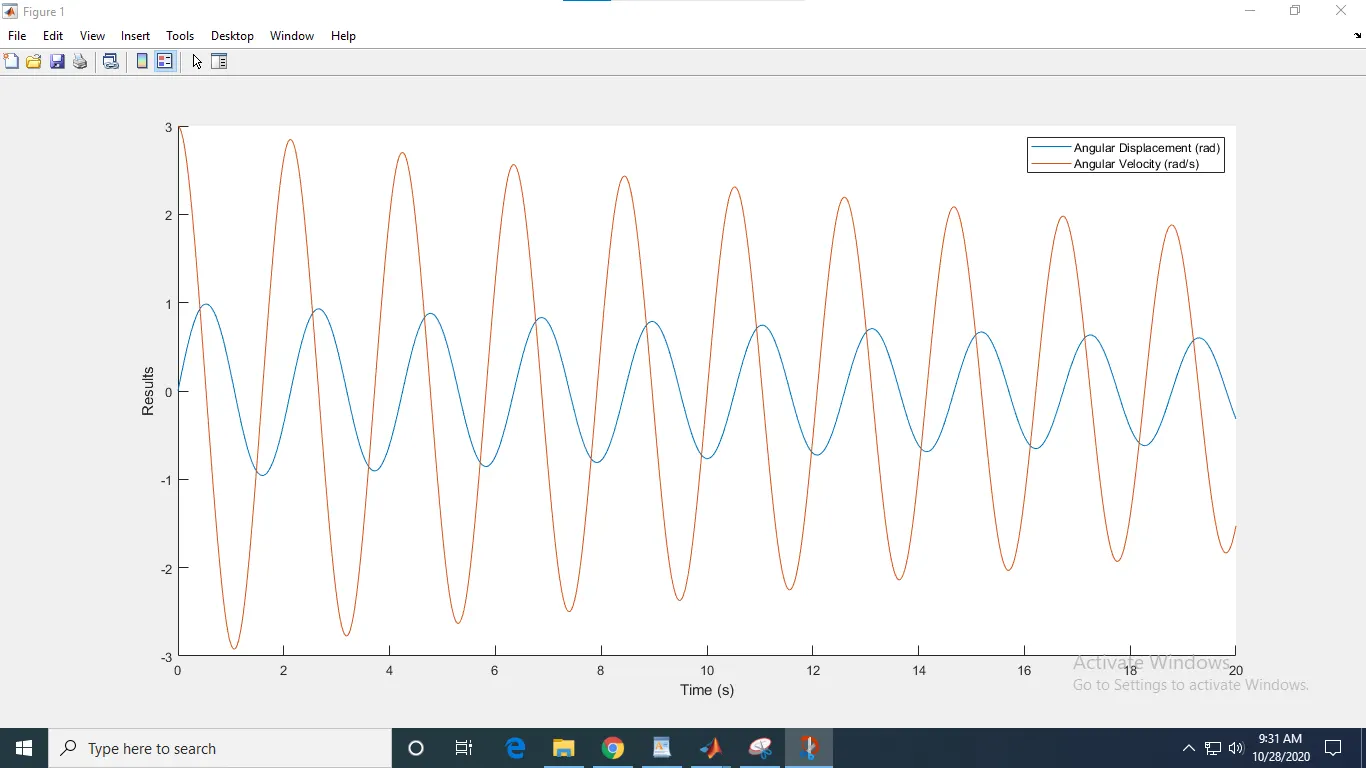
Also, the above results show that the damping (in this case drag, i.e., wind resistance and gravity) reduces the Angular velocity of the moving pendulum until it comes to it's original rest position. So, the ball will not move until and otherwise an external force is provided and hence an angular velocity of 3 rad/s is given at the initial position.
So, higher the damping coefficient in a vibrating or oscilating system, less will be the impact of angular velocity since the amplitude reduces greatly due to damping and reaches zero at a short interval of time.

The link for the 'Simple pendulum.avi' movie file is https://drive.google.com/file/d/1fw30LC68Cm_7-dK0KvrfM_AtbbzlWyYS/view?usp=sharing .