Week 5 - Mid term project - Solving the steady and unsteady 2D heat conduction problem

STUDY ON STEADY STATE & TRANSIENT ANALYSIS OF

2-DIMENSIONAL HEAT CONDUCTION EQUATION

AIM:

To study the Iterative solvers for solving the equation formed by the discretization of 2D Heat conduction PDE.

THEORY:

• Basically, there are 2 forms of PDEs which can be obtained for the 2D heat conduction equation. They are, (i) Steady State heat conduction & (ii) Unsteady State heat conduction.
• The PDE for 2D Steady state heat conduction is;

`del^2T//delx^2+del^2T//dely^2=0`

These spatial derivatives are of the Elliptic PDE Form, which can be discretized using the Central Differencing Technique. So, after discretization (2^nd order approximation), the equation becomes;

`(T_(i-1,j)-2T_(i,j)+T_(i+1,j))/(deltax^2)+(T_(i-1,j)-2T_(i,j)+T_(i+1,j))/(deltay^2)=0`

This equation is simplified for providing the solution.

• The PDE for 2D Transient or Unsteady state heat conduction is;

`delT//delt=alpha(del^2T//delx^2+del^2T//dely^2)`

In this equation, the 1^st term is the time derivative term which is of the Hyperbolic PDE form, which can be discretized using the Time Marching technique. So, after discretization, the equation becomes;

`(T_(i,j)^(n+1)-T_(i,j)^n)/(deltat)=alpha((T_(i-1,j)-2T_(i,j)+T_(i+1,j))/(deltax^2))^n+alpha((T_(i-1,j)-2T_(i,j)+T_(i+1,j))/(deltay^2))^n`

Here, the RHS terms are in the ‘n’th time step, which implies that this equation is the Explicit form of 2D Transient heat conduction equation. If the RHS terms are in the ‘n+1’th time step, then it is in the Implicit form of 2D Transient heat conduction equation. This equation is simplified for providing the solution.

• Introduction to Iterative Solvers:

To solve a system of linear equations, we can use the direct method where we set up a matrix form ‘[A][X] = [B]’ and we solve for [X] which requires only a definite number of steps to reach the solution. But, this case is not always reliable since in certain CFD problems, where we deal with millions of equations (corresponding to the mesh) which is almost impossible to solve using the direct method since it is a tedious process to code in some software. In such cases, we depend on these Iterative Solvers for solution which does not involve a definite number of steps or iterations to provide the solution, but after certain number of iterations, the values converge to the desired solution.

Basically, there are several Iterative solvers which can be used to provide the solution, but we take only 3 basic solvers into account. They are, (i) Jacobi method, (ii) Gauss-Seidel method & (iii) Successive Over Relaxation (SOR) method.

• In these iterative solvers, we assume the initial conditions for the temperature ‘T’ in a domain based on which the solver converges to provide the necessary solution with minimized errors. In case of Jacobi method, we use the assumed values of ‘T’ everywhere, while solving for the equation in every iteration. In case of GS method, we use the updated values of ‘T’ which was determined in the previous iteration for solving the present iteration equation and so on. In case of SOR method, the solution for Jacobi and GS methods can be enhanced by a factor of ‘`omega`’ which provides the results in a lesser number of iterations that the corresponding Jacobi or GS iterations.

PROCEDURE:

• In this study, the program for the 2D Heat Conduction Equation is coded using Matlab Software.

• % Program for Steady state & Transient state Analysis of 
  % 2D Heat Conduction Equation
  clear all;
  close all;
  clc;
  
  % Given Boundary Conditions;
  Tt = 600;
  Tb = 900;
  Tl = 400;
  Tr = 800;
  
  % Geometry of the frame for which heat conduction is calculated
  length = 1;
  breadth = 1;
  
  % Initializing the required Boundary conditions,
  nx = 10;
  ny = 10;
  x = linspace(0,length,nx);
  y = linspace(0,breadth,ny);
  dx = x(2)-x(1);
  dy = y(2)-y(1);
  T(1:ny,1:nx) = 300;
  T(1:ny,1) = Tl;
  T(1,1) = (Tl+Tt)/2;
  T(ny,1) = (Tl+Tb)/2;
  T(1,2:nx) = Tt;
  T(1,nx) = (Tt+Tr)/2;
  T(2:ny,nx) = Tr;
  T(ny,nx) = (Tr+Tb)/2;
  T(ny,2:nx-1) = Tb;
  
  % Steady State 2D Heat Conduction equation function
  [jacobi_error, jacobi_iter, gs_error, gs_iter, sor_gs_error, sor_gs_iter, sor_jacobi_error, sor_jacobi_iter]=steady_state_func(T,dx,dy,nx,ny,x,y);
  % 2D Transient Heat Conduction equation function
  [t_jacobi_error, t_jacobi_iter, t_gs_error, t_gs_iter, t_sor_gs_error, t_sor_gs_iter, t_sor_jacobi_error, t_sor_jacobi_iter]= transient_state_func(T,dx,dy,nx,ny,x,y);
  

• In the above main program, the given boundary conditions are provided and the necessary values for the inner BCs are assumed with respect to the dimension of the 2D frame through which heat conduction happens. For the steady and transient 2D heat conduction solution, we use 2 function programs.

• % Function program for Steady State 2D Heat Conduction Equation
  function [jacobi_error, jacobi_iter, gs_error, gs_iter, sor_gs_error, sor_gs_iter, sor_jacobi_error, sor_jacobi_iter]= steady_state_func(T,dx,dy,nx,ny,x,y)
  
  % Initializing the required terms for calculation;
  Told = T;%setting the present iteration values which are un-updated
  Tinitial = T;%used for initializing back to original T for every method
  K = 2*((dx^2+dy^2)/(dx^2*dy^2));
  tol = 1e-4;%tolerance value for which the error must be satisfied
  jacobi_error = 10;%initializing the error values
  gs_error = 10;
  sor_gs_error = 10;
  sor_jacobi_error = 10;
  jacobi_iter = 1;%to determine the number of iterations taken
  gs_iter = 1;
  sor_gs_iter = 1;
  sor_jacobi_iter = 1;
  % Steady State Jacobi method
  while(max(jacobi_error)>tol)
      for i = 2:nx-1
          for j = 2:ny-1
              term1=((Told(i,j-1)+Told(i,j+1)))/dx^2;
              term2=((Told(i-1,j)+Told(i+1,j)))/dy^2;
              T(i,j) = term1/K+term2/K;
          end
      end
      jacobi_error = max(abs(Told-T));%error calculation
      jacobi_iter = jacobi_iter+1;
      Told = T;
      figure(1);
      contourf(x,y,T);%contour plot which is filled
      xlabel('X values');
      ylabel('Y values');
      A = colorbar;
      A.Title.String = 'Temperature';%naming for colorbar
      title('Steady State Jacobi method');
      set(gca,'YDIR','reverse');%reversing the direction of y-axis
  end
  T = Tinitial;
  Told = Tinitial;
  % Steady State Gauss-Seidel Method
  while(max(gs_error)>tol)
      for i = 2:nx-1
          for j = 2:ny-1
              term1=((T(i,j-1)+Told(i,j+1)))/dx^2;
              term2=((T(i-1,j)+Told(i+1,j)))/dy^2;
              T(i,j) = term1/K+term2/K;
          end
      end
      gs_error = max(abs(Told-T));
      gs_iter = gs_iter+1;
      Told = T;
      figure(2)
      contourf(x,y,T);
      xlabel('X values');
      ylabel('Y values');
      A = colorbar;
      A.Title.String = 'Temperature';
      title('Steady State Gauss-Seidel Method');
      set(gca,'YDIR','reverse');
  end
  T = Tinitial;
  Told = Tinitial;
  % Steady State Successive Over Relaxation Method for GS
  omega = 1.05;
  while(max(sor_gs_error)>tol)
      for i = 2:nx-1
          for j = 2:ny-1
              term1=((T(i,j-1)+Told(i,j+1)))/dx^2;
              term2=((T(i-1,j)+Told(i+1,j)))/dy^2;
              T(i,j) = (1-omega)*Told(i,j)+(omega*(term1/K+term2/K));
          end
      end
      sor_gs_error = max(abs(Told-T));
      sor_gs_iter = sor_gs_iter+1;
      Told = T;
      figure(3)
      contourf(x,y,T);
      xlabel('X values');
      ylabel('Y values');
      A = colorbar;
      A.Title.String = 'Temperature';
      title('Steady State Successive Over Relaxation Method for GS');
      set(gca,'YDIR','reverse');
  end
  T = Tinitial;
  Told = Tinitial;
  % Steady State Successive Over Relaxation Method for Jacobi
  while(max(sor_jacobi_error)>tol)
      for i = 2:nx-1
          for j = 2:ny-1
              term1=((Told(i,j-1)+Told(i,j+1)))/dx^2;
              term2=((Told(i-1,j)+Told(i+1,j)))/dy^2;
              T(i,j) = (1-omega)*Told(i,j)+(omega*(term1/K+term2/K));
          end
      end
      sor_jacobi_error = max(abs(Told-T));
      sor_jacobi_iter = sor_jacobi_iter+1;
      Told = T;
      figure(4)
      contourf(x,y,T);
      xlabel('X values');
      ylabel('Y values');
      A = colorbar;
      A.Title.String = 'Temperature';
      title('Steady State Successive Over Relaxation Method for Jacobi');
      set(gca,'YDIR','reverse');
  end

• In the Steady State function, the necessary initialization which includes the ‘tolerance’ and ‘error’ values to be computed and also the ‘Told’ values which contains the values of ‘T’ in the previous iteration for all the iterations are determined. First, the Steady state equation is solved using Jacobi method where the number of iterations is determined by the Convergence loop which is the ‘while’ loop which runs until the error is lesser than the tolerance value. The error is computed by using the ‘max (abs (Told-T))’ which gives the maximum value of error which must be less than the given tolerance value for a converged solution. The ‘contour’ plot for ‘(x,y,T)’ values of all the iterations are plotted. Also, ‘set(gca,’YDIR’,’reverse’)’ command is used to reverse the Y-axis to get the rectified plot. Then, the Steady state equation is solved using GS method which involves the same procedure. Finally, the SOR method for both Jacobi method and GS method is coded similarly.

• % Function program for 2D Transient Heat Conduction Equation
  function [t_jacobi_error, t_jacobi_iter, t_gs_error, t_gs_iter, t_sor_gs_error, t_sor_gs_iter, t_sor_jacobi_error, t_sor_jacobi_iter]= transient_state_func(T,dx,dy,nx,ny,x,y)
  
  % Initializing the required terms for calculation;
  Told = T;
  Tinitial = T;
  T_prev = T;%setting T_previous values for which the next time step is used
  alpha = 1.27;%thermal diffusivity of Gold
  t = linspace(1,4,1400);
  dt = t(2) - t(1);%time step 'dt'
  K1 = alpha*dt/dx^2;
  K2 = alpha*dt/dy^2;
  tol = 1e-4;
  t_jacobi_error = 10;
  t_gs_error = 10;
  t_sor_gs_error = 10;
  t_sor_jacobi_error = 10;
  t_jacobi_iter = 1;
  t_gs_iter = 1;
  t_sor_gs_iter = 1;
  t_sor_jacobi_iter = 1;
  
  % Explicit method for Transient analysis
  for nt = 1:1400% no. of time steps
      for i = 2:nx-1
          for j = 2:ny-1
              term1=((Told(i,j-1)-2*Told(i,j)+Told(i,j+1)))*K1;
              term2=((Told(i-1,j)-2*Told(i,j)+Told(i+1,j)))*K2;
              T(i,j) = Told(i,j)+term1+term2;
          end
      end
      Told = T;
      figure(5);
      contourf(x,y,T);
      xlabel('X values');
      ylabel('Y values');
      A = colorbar;
      A.Title.String = 'Temperature';
      title('Explicit method for Transient analysis');
      set(gca,'YDIR','reverse');
  end
  T = Tinitial;
  Told = Tinitial;
  
  % Implicit method for Transient analysis
  % Jacobi method
  for nt = 1:1400
      while(max(t_jacobi_error)>tol)
          for i = 2:nx-1
              for j = 2:ny-1
                  K = (1+2*K1+2*K2)^-1;
                  term1=((Told(i,j-1)+Told(i,j+1)))*K1;
                  term2=((Told(i-1,j)+Told(i+1,j)))*K2;
                  T(i,j) = T_prev(i,j)*K+term1*K+term2*K;
              end
          end
          t_jacobi_error = max(abs(Told-T));
          t_jacobi_iter = t_jacobi_iter+1;
          Told = T;
      end
      T_prev = T;
      t_jacobi_error = 10;
      figure(6);
      contourf(x,y,T);
      xlabel('X values');
      ylabel('Y values');
      A = colorbar;
      A.Title.String = 'Temperature';
      title('Implicit method for Transient analysis-Jacobi method');
      set(gca,'YDIR','reverse');
  end
  T = Tinitial;
  Told = Tinitial;
  T_prev = Tinitial;
  
  % GS method
  for nt = 1:1400
      while(max(t_gs_error)>tol)
          for i = 2:nx-1
              for j = 2:ny-1
                  K = (1+2*K1+2*K2)^-1;
                  term1=((T(i,j-1)+Told(i,j+1)))*K1;
                  term2=((T(i-1,j)+Told(i+1,j)))*K2;
                  T(i,j) = T_prev(i,j)*K+term1*K+term2*K;
              end
          end
          t_gs_error = max(abs(Told-T));
          t_gs_iter = t_gs_iter+1;
          Told = T;
      end
      T_prev = T;
      t_gs_error = 10;
      figure(7);
      contourf(x,y,T);
      xlabel('X values');
      ylabel('Y values');
      A = colorbar;
      A.Title.String = 'Temperature';
      title('Implicit method for Transient analysis-GS method');
      set(gca,'YDIR','reverse');
  end
  T = Tinitial;
  Told = Tinitial;
  T_prev = Tinitial;
  
  % SOR for Jacobi method
  omega = 1.1;
  for nt = 1:1400
      while(max(t_sor_jacobi_error)>tol)
          for i = 2:nx-1
              for j = 2:ny-1
                  term1=((Told(i,j-1)+Told(i,j+1)))*K1;
                  term2=((Told(i-1,j)+Told(i+1,j)))*K2;
                  T(i,j) = (1-omega)*Told(i,j)+(omega*(T_prev(i,j)*K+term1*K+term2*K));
              end
          end
          t_sor_jacobi_error = max(abs(Told-T));
          t_sor_jacobi_iter = t_sor_jacobi_iter+1;
          Told = T;
      end
      T_prev = T;
      t_sor_jacobi_error = 10;
      figure(8)
      contourf(x,y,T);
      xlabel('X values');
      ylabel('Y values');
      A = colorbar;
      A.Title.String = 'Temperature';
      title('Implicit method for Transient analysis-SOR for Jacobi method');
      set(gca,'YDIR','reverse');
  end
  T = Tinitial;
  Told = Tinitial;
  T_prev = Tinitial;
  
  % SOR for GS method
  for nt = 1:1400
      while(max(t_sor_gs_error)>tol)
          for i = 2:nx-1
              for j = 2:ny-1
                  term1=((T(i,j-1)+Told(i,j+1)))*K1;
                  term2=((T(i-1,j)+Told(i+1,j)))*K2;
                  T(i,j) = (1-omega)*Told(i,j)+(omega*(T_prev(i,j)*K+term1*K+term2*K));
              end
          end
          t_sor_gs_error = max(abs(Told-T));
          t_sor_gs_iter = t_sor_gs_iter+1;
          Told = T;
      end
      T_prev = T;
      t_sor_gs_error = 10;
      figure(9)
      contourf(x,y,T);
      xlabel('X values');
      ylabel('Y values');
      A = colorbar;
      A.Title.String = 'Temperature';
      title('Implicit method for Transient analysis-SOR for GS method');
      set(gca,'YDIR','reverse');
  end

• In the Transient analysis function, along with all the necessary initialization, we give the ‘dt’ time step values as input, since the transient analysis uses time marching technique for solution. First, the explicit form of the 2D Transient heat conduction equation is solved, which does not require any iterative solvers since the solution converges with respect to time iteration itself. Then, the implicit form of 2D Transient heat conduction equation is solved for Jacobi, GS and SOR methods which follows the same procedure as above but also has a time loop to reach a steady solution without any deviation.

RESULTS:

Thus, the study on the Iterative solvers for solving the equation formed by the discretization of 2D Heat conduction PDE and the plot for the temperature ‘T’ is plotted successfully using the Matlab software.

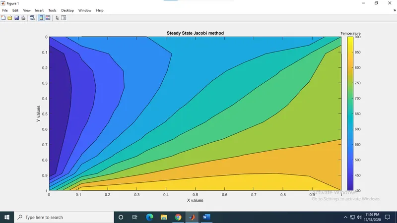
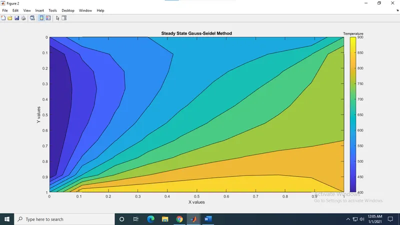
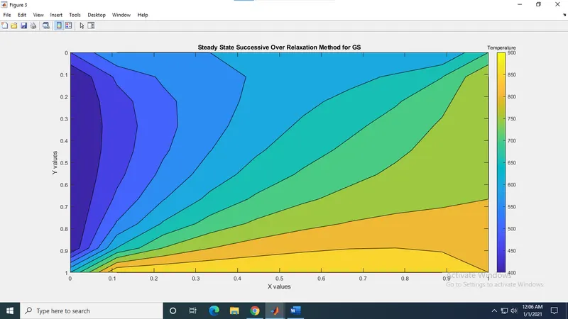
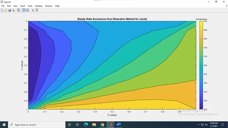
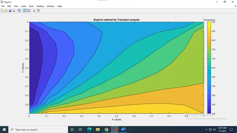
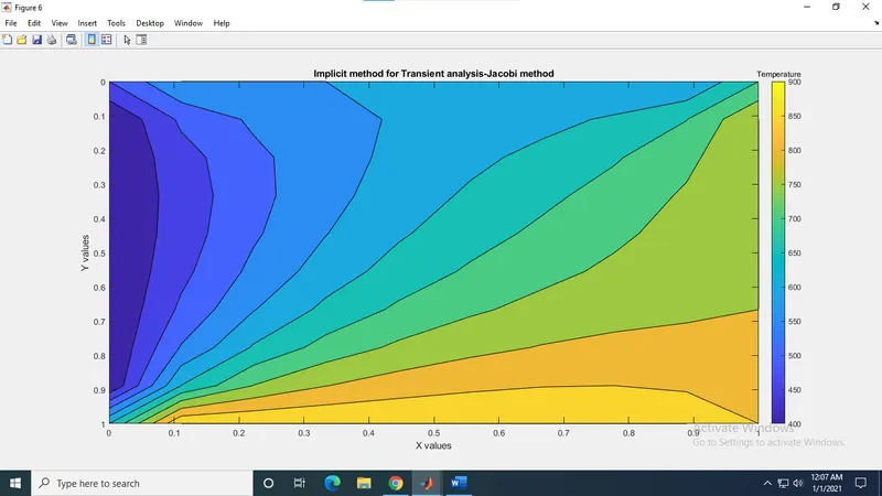
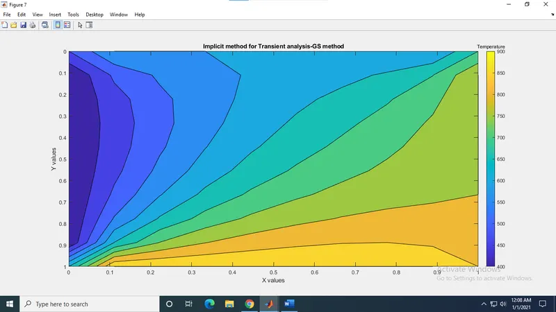
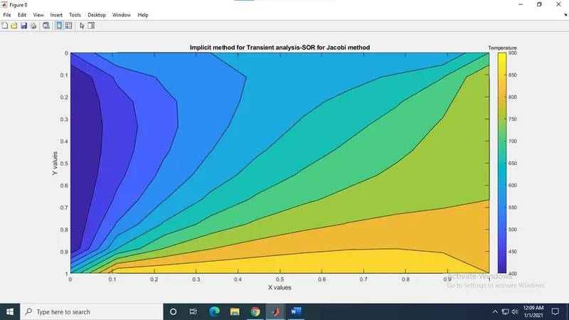
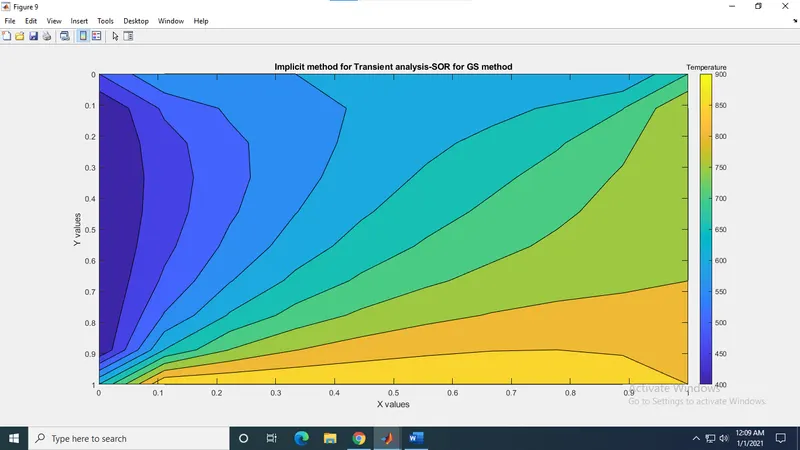
According to the above plots, we can conclude that the 2D Heat conduction equation of Steady state and Transient analysis have converged to the required results within the error tolerance limit. The only difference is that the methods that we used for obtaining theses results change due to which the number of iterations required for obtaining the solution varies. It can be observed that the number of iterations for SOR method < GS method < Jacobi method, i.e., SOR method converges to the solution faster than the other 2 methods.