Week 3 - Taylor table method and Matlab code
REPORT ON 4TH ORDER APPROXIMATION OF
2ND ORDER DERIVATIVE
AIM:
To study the purpose of Taylor Table in solving higher order derivatives and to solve a 4th order approximation of 2nd order derivative using Matlab software.
OBJECTIVES:
- To derive the 4th order approximation of 2nd order derivative of the analytical function ‘exp(x)*cos(x)’ using Central, Skewed right-sided and Skewed left-sided differencing schemes.
- To determine the Truncation error for all the 3 schemes and compare the them with each other.
- To explain the importance of Skewed scheme and why we use it.
THEORY & DERIVATION:
In this study, Central differencing takes information from equal number of nodes on the right- and left-hand side of the point f(i) or f(x). This is nothing but a Symmetric differencing scheme.
In an Asymmetric differencing scheme, it takes information from either only on the LHS or only on the RHS of the node f(i) which is called as Skewed right-sided and Skewed left-sided differencing.
We use these schemes to discretize a function and to determine the approximate values of the function at certain discrete points. In case of Central differencing, for a 2nd order of the derivative with 4th order approximation, the function goes as follows;
`f’’(x) = (a*f(i-2) + b*f(i-1) + c*f(i) + d*f(i+1) + e*f(i+2))/dx^2`
In case of Skewed right-sided scheme,
`f’’(x) = (a*f(i) + b*f(i+1) + c*f(i+2) + d*f(i+3) + e*f(i+4) + g*f(i+5))/dx^2`
In case of Skewed left-sided scheme,
`f’’(x) = (a*f(i) + b*f(i-1) + c*f(i-2) + d*f(i-3) + e*f(i-4) + h*f(i-5))/dx^2`
where, a, b, c, d, e, g and h are the coefficients that arise due to the approximation of the Taylor’s Series by ignoring some of the higher order derivatives, i.e.,
`f(i+1) or f(x + dx) = f(i) + f’(i)*dx + f’’(i)*dx^2/(2!) + f’’’(i)*dx^3/(3!) + …`
Similarly, the Taylor’s series can be taken for f(i+2), f(i-2), f(i+3) and so on.
Notations: ‘i’ indicates ‘x’ and ‘i + n’ where ‘n’ is any number is nothing but the multiplication of dx with it, for example, ‘I + 1’ is ‘x + dx’ and ‘I + 2’ is ‘x + 2dx’ and so on.
So, we can simplify the Taylor’s Series equations with the scheme equations to derive the following equation, in case of Central scheme;
Central scheme = `(a+b+c+d+e)*f(i) + (-2a-b+d+2e)*f’(i)*dx + (4a/2+b/2+d/2+4e/2)*f''(i)*dx^2+(-8a/6-b/6+d/6+8e/6)*f'''(i)*dx^3`
`+(16a/24+b/24+d/24+16e/24)*f^(iv)(i)*dx^4+O(dx^5)…`
So, in this equation, we stopped with `f^(iv)(i)` because, we have 5 coefficients and we only need 5 equations to solve them, which implies that these coefficients are equated to some value based on the order of derivative we need. Since we need a 2nd order derivative, we can equate coefficients of f(i), f’(i), f’’’(i) and f’v(i) to zero and f’’(i) to one. And by solving these equations, we can determine the Central differencing scheme. Thus, since this gets too complex for solving higher order derivatives, we take the Taylor Table method which makes things easier.
For Central Differencing Scheme, the Taylor Table is;
|
|
f(x) |
f’(x)*dx |
f’’(x)*dx^2 |
f'''(x)*dx^3 |
f'v(x)*dx^4 |
fv(x)*dx^5 |
|
a*f(i-2) |
a |
-2a |
4a/2 |
-8a/6 |
16a/24 |
-32a/120 |
|
b*f(i-1) |
b |
-b |
b/2 |
-b/6 |
b/24 |
-b/120 |
|
c*f(i) |
c |
0 |
0 |
0 |
0 |
0 |
|
d*f(i+1) |
d |
d |
d/2 |
d/6 |
d/24 |
d/120 |
|
e*f(i+2) |
e |
2e |
4e/2 |
8e/6 |
16e/24 |
32e/120 |
|
Sum |
0 |
0 |
1 |
0 |
0 |
(Ignored) |
This way it is easy to solve the derivatives and find the central scheme. It is important to notice that after summing up, the LHS becomes, `f’’(x) = a*f(i-2) + b*f(i-1) + c*f(i) + d*f(i+1) + e*f(i+2)`, so we divide the whole equation by ‘`dx^2`’ which implies that the order of equation reduces to `O(dx^3)` that is 3rd order approximation, but we claim it as 4th order approximation. This is because, upon simplification, we can see that the coefficients, a = e and b = d, so we can say from the table that the ‘`f^v(x)*dx^5`’ term does not actually exist. So, while reducing the equation, it goes up to ‘`f^(vi)(x)*dx^6`’ which when divided by ‘`dx^2`’ gets to the 4th order of approximation `O(dx^4)`. So, according to this, we can never be able to arrive at 3rd, 5th, or any other 'odd number' order of approximation for a Central differencing scheme of 2nd derivative. This is of the formula,
The order of accuracy P = Number of nodes in the stencil N - order of derivative Q + 1 for symmetric/central schemes.
Implies, N = 4+2-1 = 5 nodes for CD scheme.
Similarly, Skewed schemes can be derived like this but the only difference is that for 4th order approximation, we need 6 nodes (f(i) to f(i+5)) in total according to the formula;
The order of accuracy P = Number of nodes in the stencil N - order of derivative Q for one-sided/skewed schemes.
Implies, N = 4 + 2 = 6 nodes in case of Skewed scheme. Also, it only makes sense when we go upto ‘f(i+5)*dx^5’ because then only upon dividing by ‘dx^2’, we get the O(dx^4) accuracy.
For Skewed Right-sided Scheme, the Taylor Table is;
`f''(x)=(a*f(x)+b*f(x+dx)+c*f(x+2dx)+d*f(x+3dx)+e*f(x+4dx)+g*f(x+5dx))/dx^2`
|
|
f(x) |
f’(x)*dx |
f’’(x)*dx^2 |
f'''(x)*dx^3 |
f'v(x)*dx^4 |
fv(x)*dx^5 |
|
a*f(i) |
a |
0 |
0 |
0 |
0 |
0 |
|
b*f(i+1) |
b |
b |
b/2 |
b/6 |
b/24 |
b/120 |
|
c*f(i+2) |
c |
2c |
4c/2 |
8c/6 |
16c/24 |
32c/120 |
|
d*f(i+3) |
d |
3d |
9d/2 |
27d/6 |
81d/24 |
243d/120 |
|
e*f(i+4) |
e |
4e |
16e/2 |
64e/6 |
256e/24 |
1024e/120 |
|
g*f(i+5) |
g |
5g |
25g/2 |
125g/6 |
625g/24 |
3125g/120 |
|
Sum |
0 |
0 |
1 |
0 |
0 |
0 |
For Skewed left-sided Scheme, the Taylor Table is;
`f''(x)=(a*f(x)+b*f(x-dx)+c*f(x-2dx)+d*f(x-3dx)+e*f(x-4dx)+h*f(x-5dx))/dx^2`
|
|
f(x) |
f’(x)*dx |
f’’(x)*dx^2 |
f'''(x)*dx^3 |
f'v(x)*dx^4 |
fv(x)*dx^5 |
|
a*f(i) |
a |
0 |
0 |
0 |
0 |
0 |
|
b*f(i-1) |
b |
-b |
b/2 |
-b/6 |
b/24 |
-b/120 |
|
c*f(i-2) |
c |
-2c |
4c/2 |
-8c/6 |
16c/24 |
-32c/120 |
|
d*f(i-3) |
d |
-3d |
9d/2 |
-27d/6 |
81d/24 |
-243d/120 |
|
e*f(i-4) |
e |
-4e |
16e/2 |
-64e/6 |
256e/24 |
-1024e/120 |
|
g*f(i-5) |
g |
-5g |
25g/2 |
-125g/6 |
625g/24 |
-3125g/120 |
|
Sum |
0 |
0 |
1 |
0 |
0 |
0 |
So, upon solving the equations obtained by summing up the table, we are able to determine the coefficients a, b, c, d, e, g and h for Central, Skewed right-sided and Skewed left-sided Schemes correspondingly.
PROCEDURE:
- In this study, we will be coding a program that takes 'x' as '`pi/3`' and 'dx' in the range of '`pi/1000 to pi/40`' with 100 values in between them for the function f(x)=exp(x)*cos(x), using Matlab software.
-
% Program for 4th order approximation of 2nd order derivative clear all; close all; clc; % Input values x = pi/3; dx = linspace(pi/1000,pi/40,100); % Function that we use is f(x) = exp(x)*cos(x); fx = exp(x)*cos(x); % differentiating the function, f'(x) = ((exp(x)*(-sin(x)))+(cos(x)*exp(x)); f1x = ((exp(x)*(-sin(x)))+(cos(x)*exp(x))); % again differentiating for 2nd derivative, % f''(x) = (-(exp(x)*cos(x)+sin(x)*exp(x))+((exp(x)*(-sin(x)))+(cos(x)*exp(x))); % Simplifying, analytical_derivative = -2*exp(x)*sin(x); % Now, we determine the 4th order approximation of various differencing scheme; % Function call for Central differencing error1 = central_approx_O4_for_2nd_derivative(x, dx, analytical_derivative); % Function call for Skewed right-sided differencing error2 = skewed_right_O4_for_2nd_derivative(x, dx, analytical_derivative); % Function call for Skewed left-sided differencing error3 = skewed_left_O4_for_2nd_derivative(x, dx, analytical_derivative); % 'loglog' command is used to create a meaningful plot in which the x and y % values differ enormously. loglog(dx,error1,'linewidth',3); hold on; loglog(dx,error2,'linewidth',3); loglog(dx,error3,'linewidth',3); xlabel('Values for dx'); ylabel('Error'); legend('Central differencing error','Skewed right-side error','Skewed left-side error','location','southeast') title('Discretization of 2nd order derivative with 4th order approximation'); - In the above program, the function f(x) is differentiated twice to get the second order derivative f’’(x), which can be used to calculate the analytical derivative of that function. Then, using the 3 Schemes, we can determine 3 error terms Central error, Skewed right-sided error and Skewed left-sided error. Finally, a plot using ‘loglog()’ command is made with values of ‘dx’ and ‘errors’ along x & y-axes respectively. The ‘loglog()’ command is used to provide a meaningful plot for the values where the range of variance of error1, error2 and error3 is so large that it cannot be clearly understood in a single plot command.
-
% Function program for 4th order approx. of 2nd derivative Central differencing function error1 = central_approx_O4_for_2nd_derivative(x, dx, analytical_derivative) % First we need to determine the coefficients of the discretization of % the 2nd order derivative 4th order central differencing; % f''(x)=(a+b+c+d+e)f(x)+(-2a-b+d+2e)f'(x)dx+(4a/2+b/2+d/2+4e/2)f''(x)dx^2 % +(-8a/6-b/6+d/6+8e/6)f'''(x)dx^3+(16a/24+b/24+d/24+16e/24)f''''(x)dx^4; % This equation is derived using taylor table method, so to determine % a,b,c,d,e we need to solve the below matrix; A = [1 1 1 1 1;-2 -1 0 1 2;4/2 1/2 0 1/2 4/2;-8/6 -1/6 0 1/6 8/6;16/24 1/24 0 1/24 16/24]; B = [0;0;1;0;0]; C = A\B;% '\' indicates that the inverse of A matrix multiplies with B, implies C=B*A^-1; % Now we can apply these coefficients in the algebraic equation, % f''(x)=(af(x-2dx)+bf(x-dx)+cf(x)+df(x+dx)+ef(x+2dx))/dx^2; for i=1:length(dx) central_differencing(i) = (C(1,1)*(exp(x-(2*dx(i)))*cos(x-(2*dx(i))))+C(2,1)*(exp(x-dx(i))*cos(x-dx(i)))+C(3,1)*(exp(x)*cos(x))+C(4,1)*(exp(x+dx(i))*cos(x+dx(i)))+C(5,1)*(exp(x+(2*dx(i)))*cos(x+(2*dx(i)))))/dx(i)^2; % Error calculation for Central scheme; error1(i) = abs(central_differencing(i) - analytical_derivative); end end -
% Function program for 4th order approx. of 2nd derivative Skewed right-side differencing function error2 = skewed_right_O4_for_2nd_derivative(x, dx, analytical_derivative) % First we need to determine the coefficients of the discretization of % the 2nd order derivative 4th order approximation for skewed right-side differencing; % The equation is derived using taylor table method, so to determine % a,b,c,d,e,g we need to solve the below matrix; A = [1 1 1 1 1 1;0 1 2 3 4 5;0 1/2 4/2 9/2 16/2 25/2;0 1/6 8/6 27/6 64/6 125/6;0 1/24 16/24 81/24 256/24 625/24;0 1/120 32/120 243/120 1024/120 3125/120]; B = [0;0;1;0;0;0]; C = A\B; %'\' indicates that the inverse of A matrix multiplies with B, implies C=B*A^-1; % Now we can apply these coefficients in the algebraic equation, % f''(x)=(af(x)+bf(x+dx)+cf(x+2dx)+df(x+3dx)+ef(x+4dx)+gf(x+5dx))/dx^2; for i=1:length(dx) skewed_right_side(i) = (C(1,1)*(exp(x)*cos(x))+C(2,1)*(exp(x+dx(i))*cos(x+dx(i)))+C(3,1)*(exp(x+(2*dx(i)))*cos(x+(2*dx(i))))+C(4,1)*(exp(x+(3*dx(i)))*cos(x+(3*dx(i))))+C(5,1)*(exp(x+(4*dx(i)))*cos(x+(4*dx(i))))+C(6,1)*(exp(x+(5*dx(i)))*cos(x+(5*dx(i)))))/dx(i)^2; % Error calculation for Skewed-right scheme; error2(i) = abs(skewed_right_side(i) - analytical_derivative); end end -
% Function program for 4th order approx. of 2nd derivative Skewed left-side differencing function error3 = skewed_left_O4_for_2nd_derivative(x, dx, analytical_derivative) % First we need to determine the coefficients of the discretization of % the 2nd order derivative 4th order skewed left-side differencing; % The equation is derived using taylor table method, so to determine % a,b,c,d,e,g we need to solve the below matrix; A = [1 1 1 1 1 1;0 -1 -2 -3 -4 -5;0 1/2 4/2 9/2 16/2 25/2;0 -1/6 -8/6 -27/6 -64/6 -125/6;0 1/24 16/24 81/24 256/24 625/24;0 -1/120 -32/120 -243/120 -1024/120 -3125/120]; B = [0;0;1;0;0;0]; C = A\B; %'\' indicates that the inverse of A matrix multiplies with B, implies C=B*A^-1; % Now we can apply these coefficients in the algebraic equation, % f''(x)=(af(x)+bf(x-dx)+cf(x-2dx)+df(x-3dx)+ef(x-4dx)+hf(x-5dx))/dx^2; for i=1:length(dx) skewed_left_side(i) = (C(1,1)*(exp(x)*cos(x))+C(2,1)*(exp(x-dx(i))*cos(x-dx(i)))+C(3,1)*(exp(x-(2*dx(i)))*cos(x-(2*dx(i))))+C(4,1)*(exp(x-(3*dx(i)))*cos(x-(3*dx(i))))+C(5,1)*(exp(x-(4*dx(i)))*cos(x-(4*dx(i))))+C(6,1)*(exp(x-(5*dx(i)))*cos(x-(5*dx(i)))))/dx(i)^2; % Error calculation for Skewed-left scheme; error3(i) = abs(skewed_left_side(i) - analytical_derivative); end end - In the 3 function programs, we use the Taylor Table for the 3 Schemes in order to determine the coefficients of those respective scheme and with those coefficients, we can determine the 4th order Numerical Solution using the formula. The corresponding error values for the 3 schemes are also calculated using the formula, error = abs(Differencing Scheme – Analytical Derivative), where ‘abs’ means the absolute value of the difference.
RESULTS:
Thus, the study on Central Skewed right-sided and Skewed left-sided Schemes for 4th order approximation of 2nd order derivative is completed successfully using Matlab software.
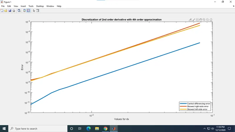
In the above plot, it is clear that the accuracy of Central Differencing Scheme is greater than the accuracy of Skewed right or left Schemes but the CD scheme cannot be applied at all the instance, for example, in case of discretization at the Boundaries of a geometric profile, we cannot get the information of the points beyond the boundary, so only Skewed schemes can be applied in this case since the CD scheme requires points or nodes to be present on both the sides. So, CD scheme is also known as Unbounded Scheme.
Moreover, discretization of a function derivative which is at a steady state of motion requires for the Skewed schemes for approximation (even though the accuracy might be low), because in this case, if we apply CD scheme, there are certain oscillations or disturbances produced while simulating in CFD which can take away the solution to be completely wrong, whereas and Up winded skew scheme can provide a relatively lower accurate solution, but the results are more stable than CD scheme. So, this tells us the importance of Skewed schemes in discretization.