Week 8 - Simulation of a backward facing step in OpenFOAM

STUDY ON SIMULATION OF

BACKWARD FACING STEP

AIM:

To simulate an incompressible-laminar-viscous flow through a backward facing step geometry using OpenFOAM software.

OBJECTIVES:

• To perform a transient simulation for flow of the incompressible viscous fluid through a backward facing step profile.
• To simulate the flow without any Grading Factor, i.e., GF = 1.
• To simulate the flow with a Grading Factor of 0.2. The cells should be finer near the walls.

PROCEDURE:

• In this study, first we need to set-up the simulation in openFOAM with all the necessary inputs.
• At First, the geometry of a backward facing step must be created in OpenFOAM. For that we need to determine the vertices. Before all that, in OpenFOAM tutorials folder, we need to determine which file is the correct match for our flow problem in order to derive a solution. So, inside terminal command box, under “tutorials” folder, by navigating into the “incompressible” folder à into the “icofoam” folder (for incompressible flow problems), “cavity” folder is chosen for this problem. It is copied into the “$OPENFOAM_RUN” directory.
• 
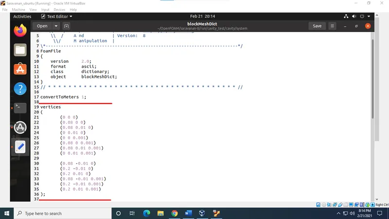
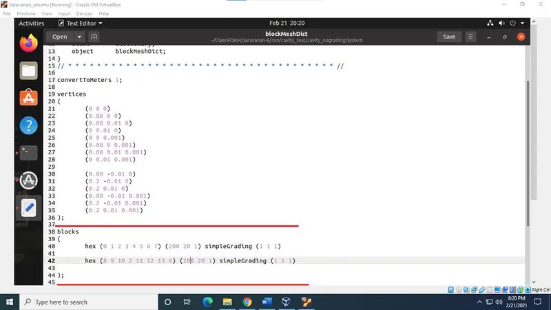
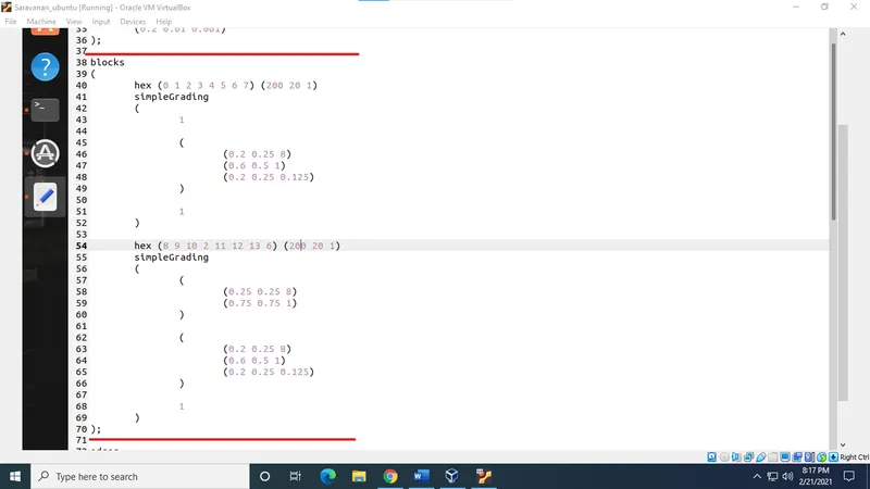
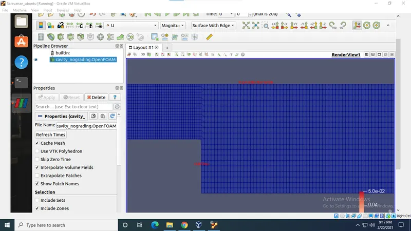
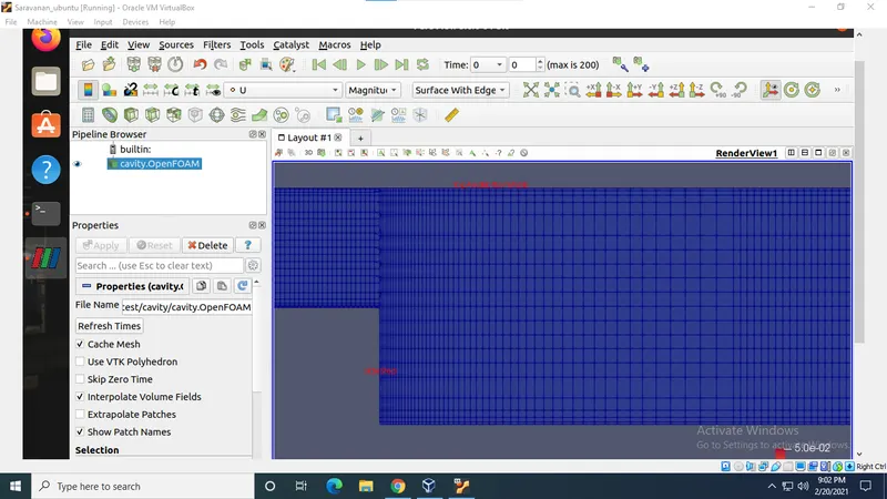
• Now to create the vertices of the geometry, we need to determine the number of blocks required to create this geometry. I chose 2 blocks to form the backward facing step. Then we need to determine the vertices of the blocks in the “blockMeshDict” file, inside the “system” folder. After that, the blocks are defined with the type of mesh, number of mesh along the x,y & z directions and the Grading Factor for the mesh inside the ‘block’ section. For case_1, the Grading factor is 1 with a ‘simpleGrading’ keyword and hexahedral mesh is chosen for this problem. For case_2, the GF = 0.2 with ‘simpleGrading’ and also with hexahedral mesh with 200 cells along x-direction and 20 cells along y-direction. Since this is a 2D simulation, there is no necessary to give more than 1 cell along the z-direction because it is not used.
• 
• 
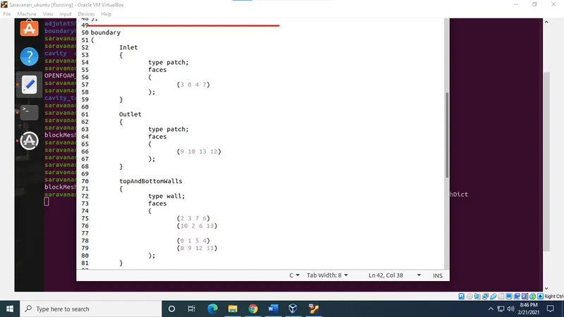
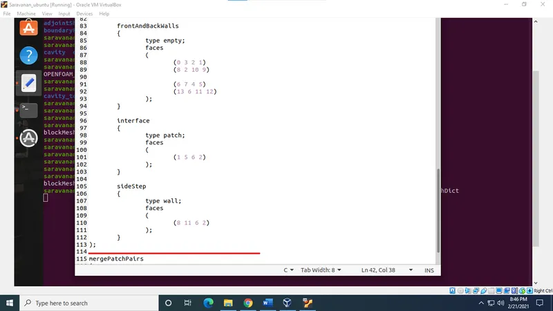
• Now after the geometry creation, the boundary conditions need to be applied to all the boundaries of the geometry. This is done in the ‘boundary’ section of the “blockMeshDict” file, where the top, bottom and sidestep are given the type ‘wall’ which indicates that the condition is ‘no slip’ (velocity is zero). The front and back faces of the geometry is given ‘empty’ since z-direction is neglection in 2D simulation. The inlet, outlet and interface between 2 blocks is given a type ‘patch’ since we need the flow to happen through these faces. In “mergePatchPairs”, we can join the 2 blocks with the interface patch which creates continuity of mesh from one block to the next.
• 
• 
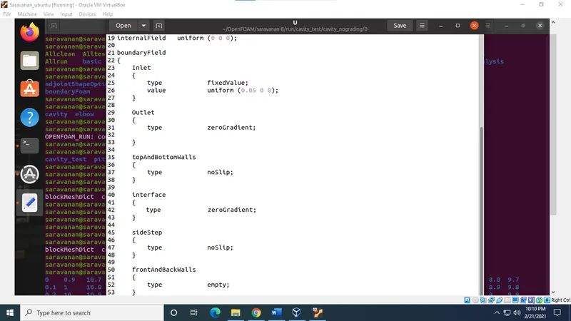
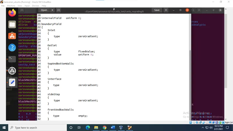
• Now we need to determine the initial conditions and the constant properties of this problem. For initial conditions, i.e., at time step 1, where t = 0, navigate to the “0” folder and edit the “U” and “p” flow properties. In this problem the initial velocity is set to uniform 0.05 m/s at the inlet and an initial pressure of uniform 0 bar gauge-pressure (1atm pressure) outlet. So, it is a velocity inlet and pressure outlet problem. The only constant parameter is `nu`, which is the kinematic viscosity of the viscous fluid and it is equal to 1e-6 in our case.
• 
• 
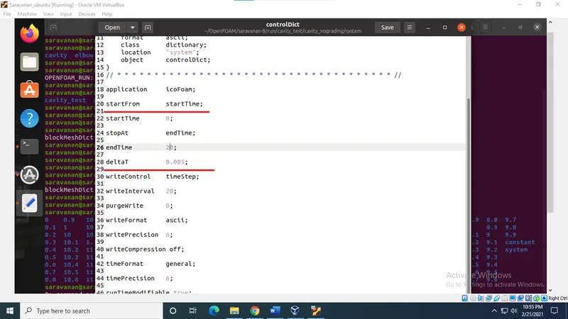
• Now for stability of flow, the CFL number is kept within limit by having a low value for `Deltat` = 0.005 and the time limit is set to 20 seconds for which steady state is reached for this problem. This is done in the “controlDict” file.
• 
• Now, it is ready for simulation. The process to start the simulation is to get in the folder where all the files are present and to create the meshed block, we need to type “blockMeshDict” in terminal in that folder and in order to start the calculation process, type in “icoFoam”. Once the program comes to an end, we can view the simulation by using “paraFoam” which essentially opens up ‘paraview’ in OpenFOAM.

RESULTS:

Thus, the simulation of an incompressible-laminar-viscous flow through a backward facing step geometry using OpenFOAM software is successfully conducted.

The results of the meshed geometry are as follows;

Case_1:

Case_2:

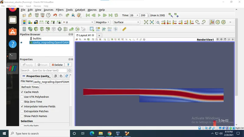
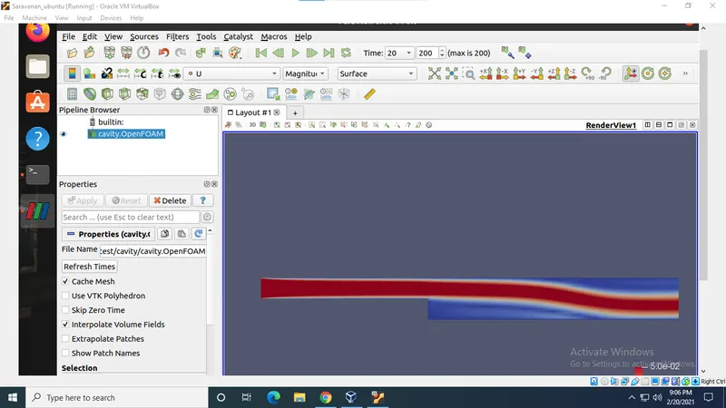
The results after simulation;

Case_1:

Case_2:

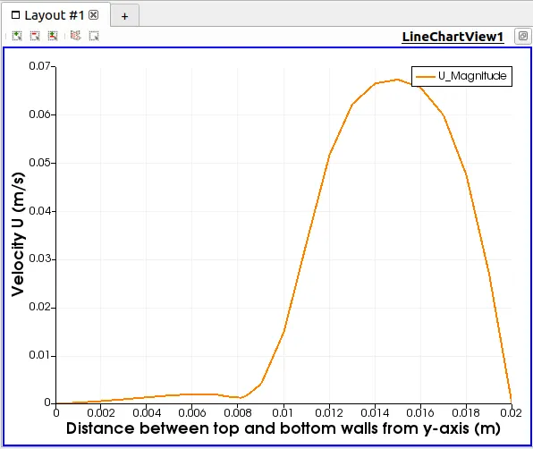
Velocity profile at a distance 0.085 m from inlet for;

Case_1:

Case_2:

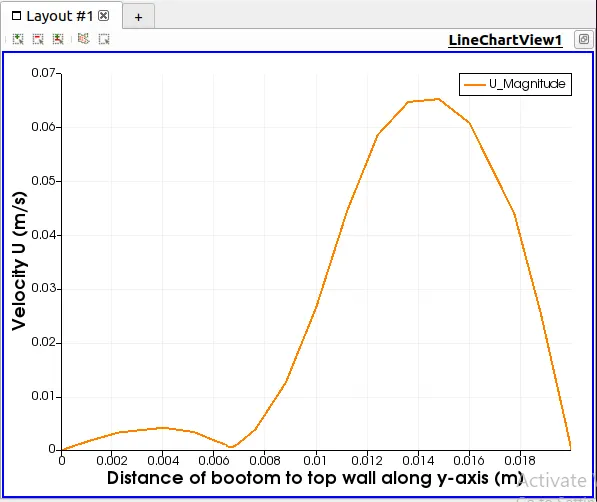
Grading or Growth Factor is necessary for mesh process since it determines the accuracy of the results. Also, in order to capture the physical parameters of the fluid flow at and near the walls, we need finer mesh near the walls so as to obtain more precise results. As we can observe in the above plots, where in case_1, there is no grading given so the velocity near the wall is not as significant when compared with case_2 which provides us with a clear picture of the effect of side step in the disturbance of the velocity of the fluid which is an important phenomenon for study.

The physical phenomena involved in this problem are Poiseuille’s law for laminar flow upto 0.08 m of flow and after that laminar flow experiences a disturbance due to the pressure difference from block 1 to 2 since there is a drop in the pressure gradient along x-direction due to which the discharge of the flow becomes random (vortex or whirl flow creation) for a certain period of time till the flow reaches steady state. So, at 0.085 m, it might be considered as the transition region of flow separation. Also, this flow will reach steady state since we consider a real time viscous flow to take place.