Week 8 - Simulation of a backward facing step in OpenFOAM

Simulation of a Backward-Facing Step in OPENFOAM:

Aim: 1. Simulate an incompressible-laminar-viscous flow through the backward facing geometry.

2. Perform transient simulation; choose solver based on the desired physics of the flow in the problem statement.

3. Explain simulation process and way of setting up the problem in OPENFOAM and also, explain every change that has been done inside the reference case files obtained from OPENFOAM tutorials.

4. Next, perform two case studies, firstly, form simulation of the flow without using any grading factor. Secondly, simulate the flow with grading factor of 0.2. The cells should be finer near the walls.

Objectives: 1. Open OPENFOAM tutorial and find the solver to solve incompressible-laminar-viscous flow problem.

2. Next step is to copy required file in solver and paste it in OPENFOAM run folder so that the official file of OPENFOAM remains untouched.

3. Find out block mesh script file to create domain space and provide mesh specification.

4. Find 'controlDict' file to edit start and end time for simulation.

5. In initial folder 'O', edit initial parameter for velocity and pressure according to faces of the given domain.

6. Use blockMesh command to generate mesh and checkMesh to verify it. Open simulation file in paraView and plot the velocity profile at point 0.085m from inlet. Repeat above procedure for grading factor 0.2 to check the differences in results and finally, write a report explaining all the codes and commands used in this project.

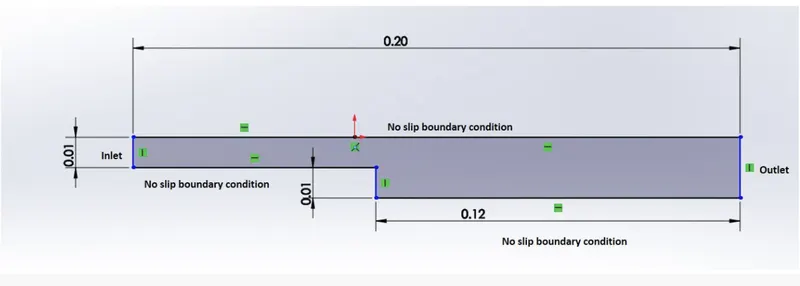
Problem Statement: Simulate an incompressible-laminar-viscous fow through the backward-facing step geometry and perform two case studies as described below and compare the results.

Case 1: Simulate the flow without using any grading factor i.e. G.F=1.

Case 2: Simulate the flow with a grading factor of 0.2. The cells should be finer near the walls(including the step wall).

Mesh Specification: 1. No. of cells along the x-direction(longer dimension)=200.

2. No. of cells along the longer y-direction=20.

Boundary Condition Specification: The domain specifications are provided in the following figure:

Simulation Process:

1. In order to start the simulation process, first fire up the terminal in Linux OS using ctrl+alt+T buttons on keyboard or right click: Open Terminal. After starting terminal, the below window will be seen:

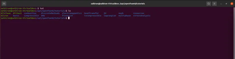
2. Now, we have to simulate our problem in OPENFOAM and we are going to solve our problem using the tutorial present in OPENFOAM, so just type 'tut' to open OPENFOAM tutorial directory and type 'ls' to identify what kind of tutorials are available in the directory.

3. We have to solve incompressible flow simulation for this problem, so select the incompressible directory by typing 'cd incompressible' and then again type 'ls' to explore folders in that.

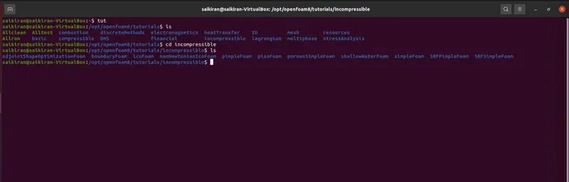
4. In the above picture, we can see many solver folders. For this particular solver, we need a solver for laminar-viscous flow. So, choose icofoam which can be used as a transient solver for incompressible and laminar flow of newtonian fluids. Thus, we will select icofoam folder by typing 'cd icoFoam' and typing 'ls' to explore folders. Next, we have to choose between 'cavity' or 'elbow'. Both are used to create required domain and black mesh, so select 'cavity' folder.

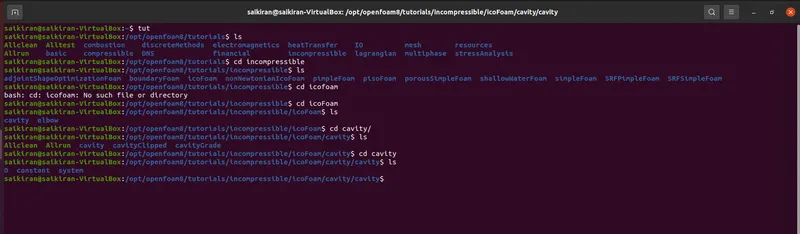
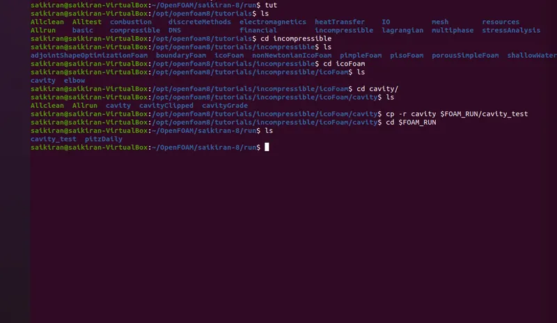
5. In 'cavity',we are again going to see the cavity folder where we have to define our fluid domain and generate blockmesh, but we're not going to make any changes here because OPENFOAM does not let anyone make changes in their official tutorial because it might corrupt the system. So, we're going to copy this cavity folder using 'cp -r cavity' command and paste it in OPENFOAM run folder by typing 'cp -r cavity' $FOAM_RUN/cavity_test' and then open folder by typing 'cd $FOAM_RUN' where we can see the cavity test file.

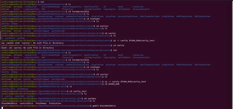
6. Now, we can make changes to the 'cavity_test' file which won't affect the official files. Open the cavity_test folder and here, we provide specification for our block mesh in system folder. There are 4 script files system folders in the below picture and by opening blockMeshDict, we can create domain and provide required specification for block mesh. So, open the file by typing 'gedit blockMeshDict'.

7. Now make following changes in blockMeshDict script file. It is a script file that contains information regarding all aspects of geometry.

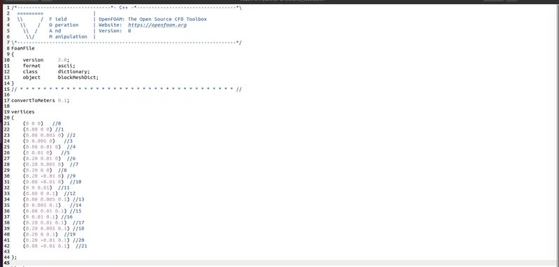
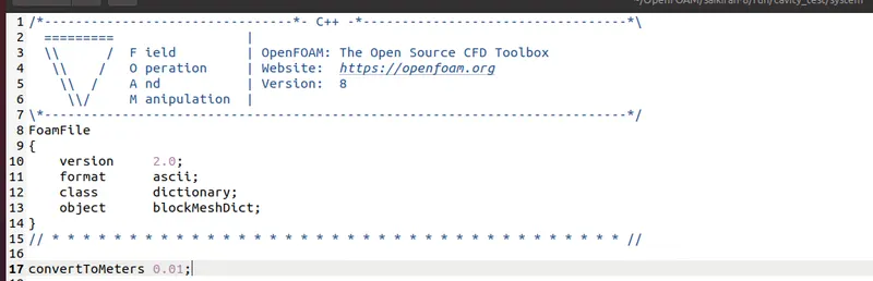
8. When we open the file, first we are going to see header information in the form of comment which is inexecutable. Then, we will see the file identifier by which OPENFOAM reads to understand the type of file its reading , in this case it is 'blockMeshDict' which contains information in the dictionary format, means key and value format. As we can see version is the key and '2.0' is its value and thats why its called 'key-value pair'. Here, we don't make any changes. Finally, we set units in meters by converting all types of length to meter.

Mesh Generation Without Any Grading Factor:

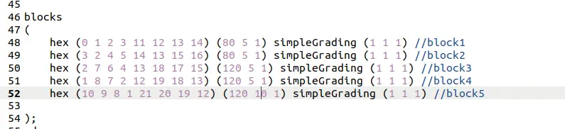
In the same blockMesh files, go to the lines where the word 'hex' can be found. That is the line where we specify the faces of the blocks and also the number of cells in X,Y and Z direction.

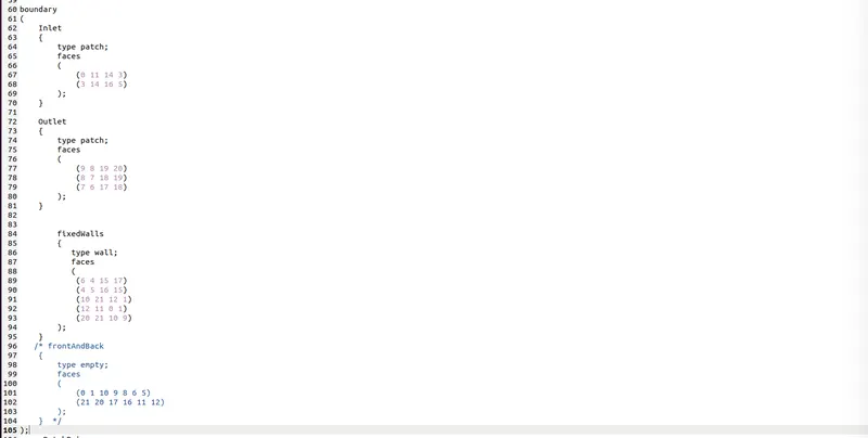
Also, we specify the faces as the inlet, outlet and walls shown in the image below:

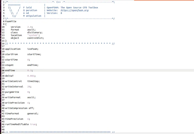
The blockMeshDict file is edited as shown above. The next step is to navigate the controlDict folder and specify the simuation time as 200 seconds. The script file looks as follows:

Vertices: Afterwards, in codes, we provide list of vertices by providing x, y and z coordinates locations; it always starts from vertex(0,0,0), so we have to create following geometry.

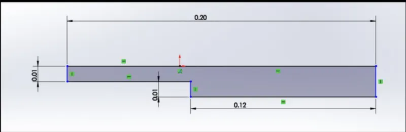
To create the above geometry, let us consider creating the geometry using 5 blocks as exhibited in below figure:

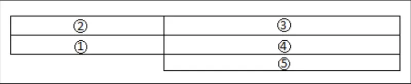
Now, we're going to provide vertices for each block by referring following sketch:

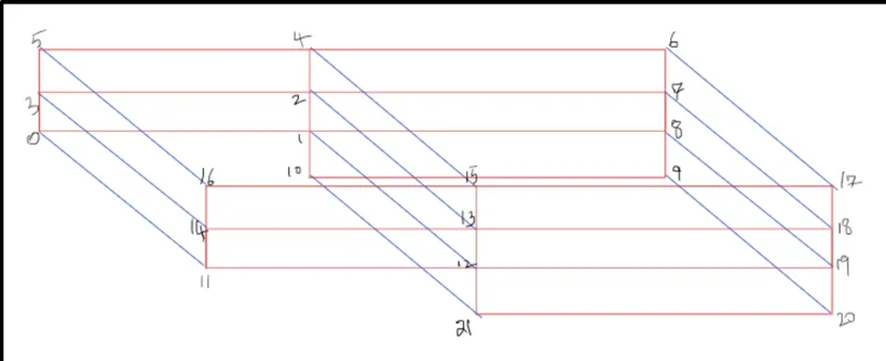
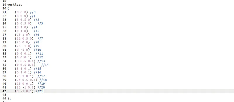
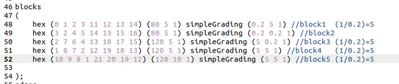
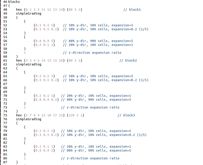
Next, we are going to define block for meshing. If we look at the mesh format first letter, in block parantheses, is 'hex' which defines type of mesh which is hexahedral mesh. Then, again in parantheses, we provide vertices number according to order which follow right hand thumb rule, meaning, thumb is the 'z' axis and order of vertices follow rotational order of other fingers. Then, comes no. of mesh grid that we want to divide along 'x','y' and 'z' length. We define it as (nx,ny,nz) format.

Given Mesh Specification: 1. No. of cells along the 'x' direction(longer dimension)=200.

2. No. of cells along the longer 'y' direction=20.

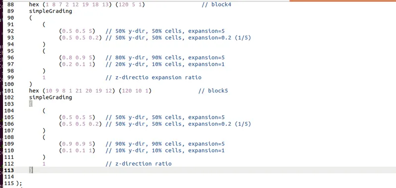
Lastly, we give simple grading which is cell expansion ratios.

Grading Factor or Expansion Ratios: The expansion ratios enable the mesh to be graded or refined in specified directions. The ratio is that of the width of the end cell `delta_e`along one edge of a block to the width of the start cell `delta_s`along the edge as shown in figure.

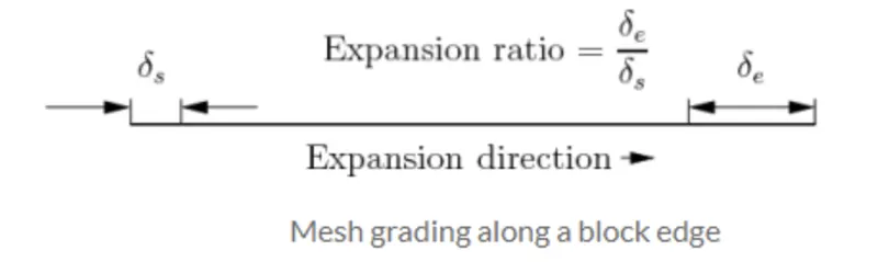
In simple format, Expansion Ratio=(Size of End Cell)/(Size of Starting Cell)

The simple description specifies uniform expansion in the local `x_1,x_2 and x_3`directions respectively with only 3 expansion ratios. For first case, we are not going to provide any grading for our problem.

So, here, we have 5 blocks, so we have to define hex mesh for 5 blocks.

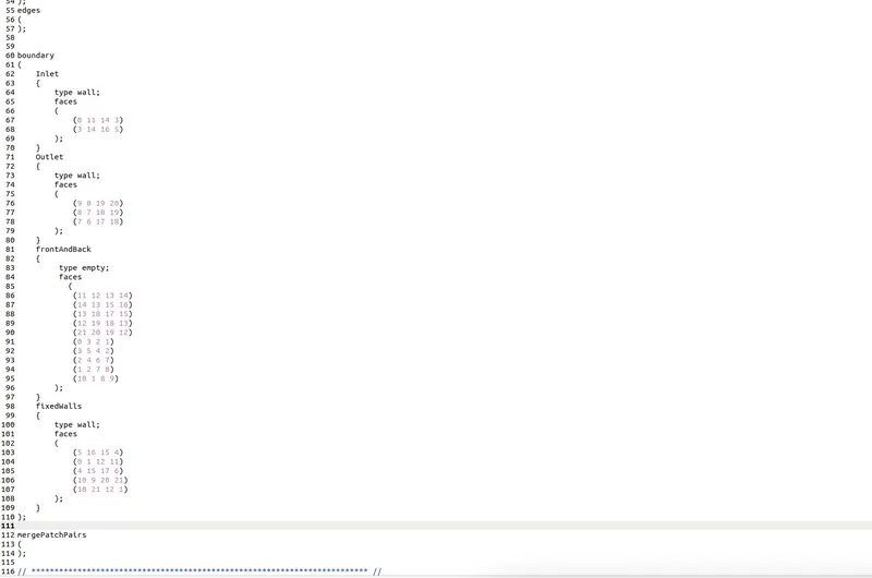
Next, define the boundary of the problem, in this way we have to define the faces of our 3D block. This should be in order according to right hand thumb rule. So set faces for this problem following way.

After editing of blockMeshDict file, save it and close it. Furthermore, we are going to edit 'controlDict' file to provide time limits(start time and end time), also to represent deltat. While selection of deltat, CFL value should be less than 1, otherwise the solution could stop forcibly or it may diverge at the time of converging, so make following changes in 'controlDict' file.

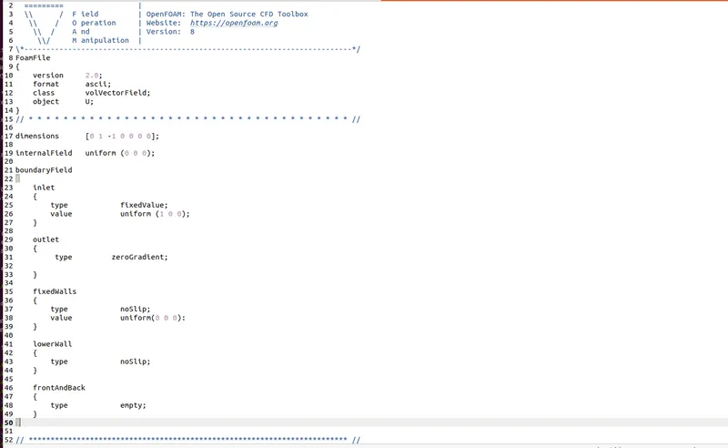
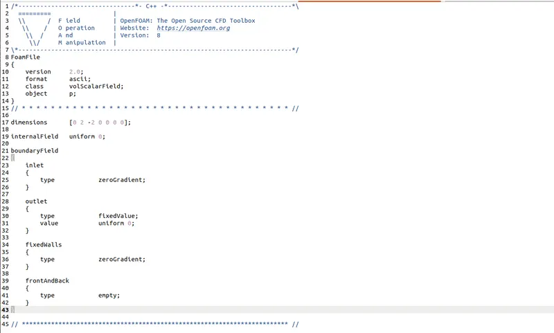
Then, we have to define initial value for pressure and velocity. In order to do that, we have to go back to cavity_copy directory using 'cd..' command and select folder named '0', which stand for initial values, in this case for pressure and velocity. Next, we have to set initial boundary conditions for pressure and velocity at each faces and also update the name of the boundary same as we changed inlet outlet name 'blockMeshDict' script file as shown below:

Initial Velocity Setting:

Initial Pressure Setting:

At this point our problem statement is set, we can now proceed to deploy mesh using 'blockMesh' command and then use 'checkMesh' command to check if there are any errors in the mesh. After checking the mesh, we get the confirmation seen in the bottom most image.

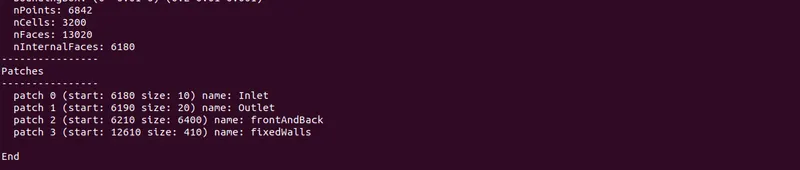
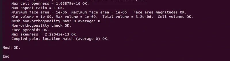
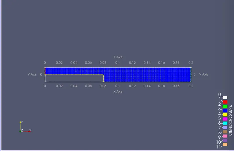
Type 'paraFoam' command to view the mesh and to check whether it is according to requirement.

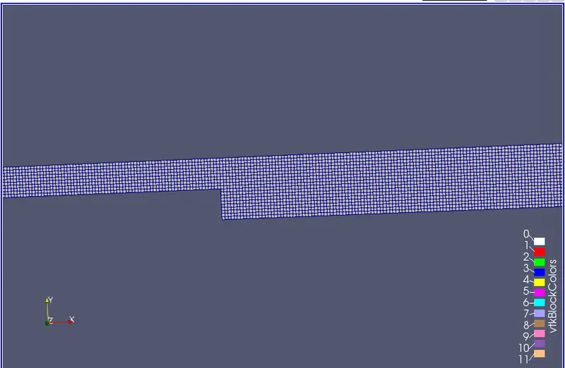
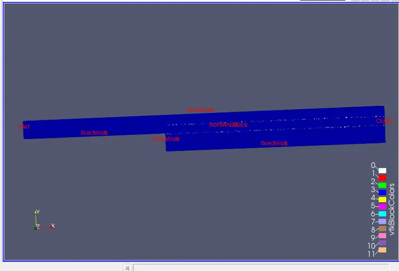
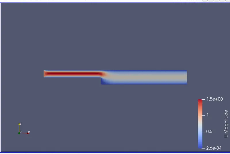
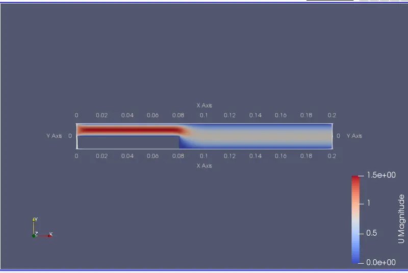
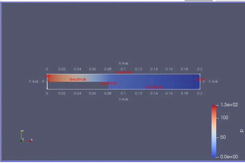
Velocity Distribution Along Domain Area:

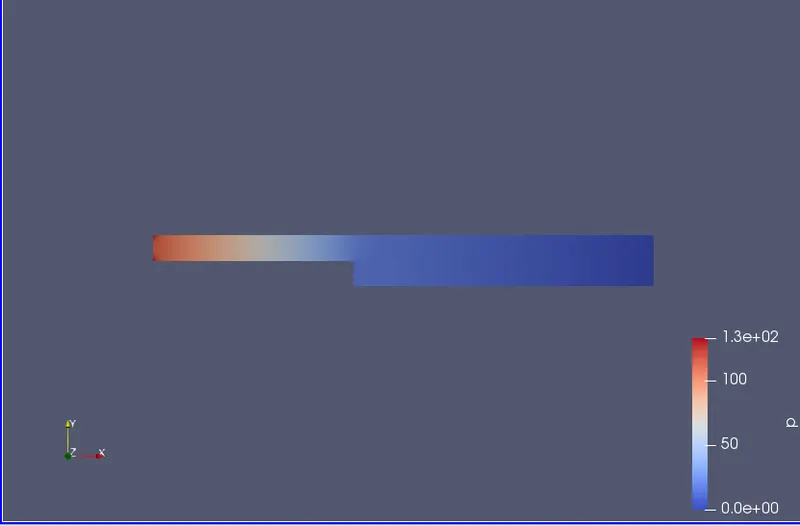
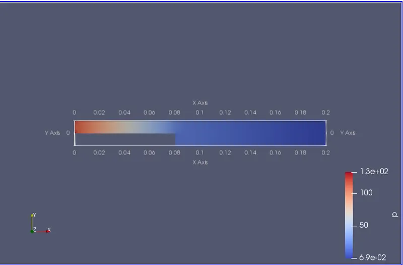
Pressure Distribution Along Domain Area:

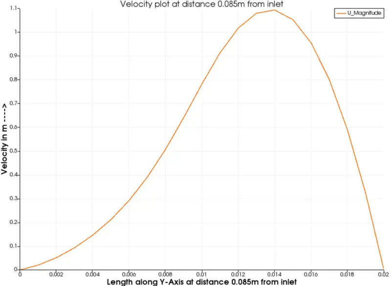
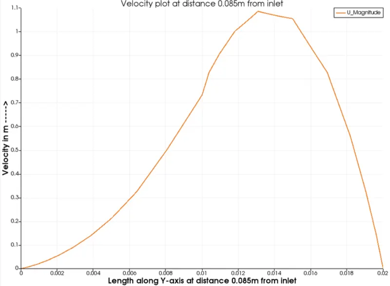
Velocity Plot:

With Grading Factor 0.2(cell near fixed walls):

Now, lets solve the same problem for grading factor 0.2

Output Mesh From Above Codes:

Velocity Distribution Along Domain Area:

Pressure Distribution Along Domain Area:

Velocity Plot:

With Grading Factor 0.2(cell near all walls):

Next, use grading factor 0.2 for all walls in the system:

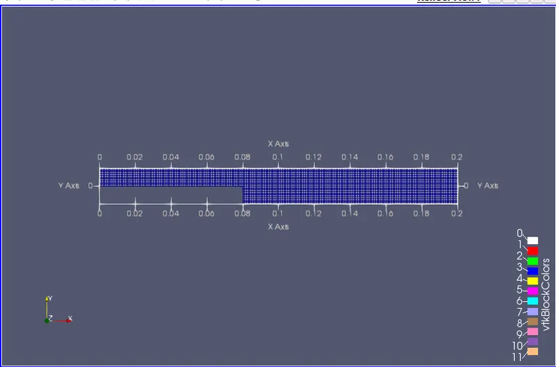
Output Mesh From Above Codes:

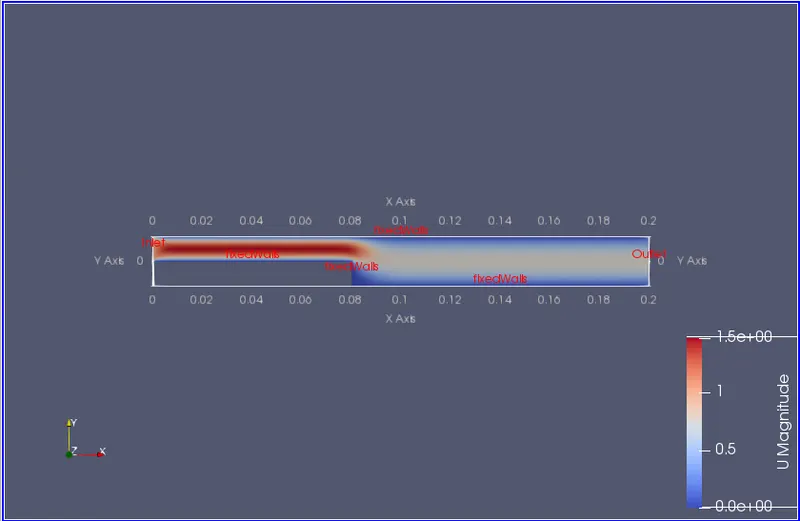
Velocity Distribution Along Domain Area:

Pressure Distribution Along Domain Area:

Velocity Plot:

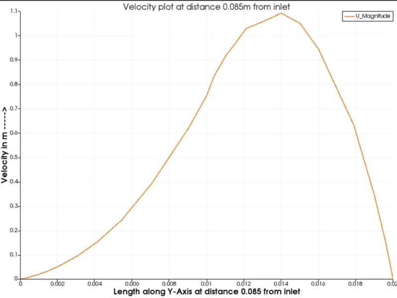
Results:Up to this point, we are done with the plotting of velocity for both: without grading factor and with grading factor '0.2'. If we take a look at all 3 velocity plots, we can see that the plot for velocity without the grading factor seems more smoother and accurate when compared to the other two plots. So, one can infer that grading inclusion disrupts the results and the outputs, but it is incorrect, if we take a look at it, we will notice that the mesh is fine at step wall along the X-axis, but coarser along the Y-axis. Thus, we 're not getting a smooth velocity plot for 0.085 point at Y-axis. Therefore, on a more conclusive note, if we were to compare all 3 plots, we would infer that inclusion of a certain value for grading factor may induce less smooth plots, but in CFD, we will always find large changes near walls and obstacles and in a bid to capture the changes effectively, we use the concept of 'grading' or finer meshes.

To get effective and reliable results, one should know where to use finer grading factor. In a bid to attain effective results, suppose if we use large no. of fine elements, it could use our computation time and also require large memory(RAM). Therefore, use of grading is important, so that we can use fine mesh to captute the flow at the boundary wall and obstacles, course mesh at more open area. Furthermore, increase in grading factor near step improves the resolution. Hence, grading/growth factor is essential for smooth meshing.