Week 7 - Simulation of a 1D Super-sonic nozzle flow simulation using Macormack Method
Aim: Simulating quasi 1D supersonic flow through a converging-diverging nozzle using MacCormack method.
Objective: 1. Deducing the conservative and non-conservative forms of governing eqns. and implementing MacCormack method to solve the eqns. and comparing the results.
2. Comparing the steady-state distribution of fluid variables in the nozzle and the time variation of the variables.
3. Studying the variation of mass-flow rate inside the nozzle at different time steps under the influence of time marching.
Theory: A nozzle is a type of device designed to control the direction or characteristics of fluid flow at the exit of a pipe. A nozzle is often a pipe or tube of varying cross-sectional area and thus can be used to direct or modify fluid flow. A covergent-divergent nozzle(CD nozzle) is a device used to accelerate a hot, pressurized gas passing through it to a higher supersonic speed in the axial direction by converting heat energy of flow to kinetic energy. Hencer, such nozzles are widely used in steam turbines, rocket engine nozzles and supersonic jet engines. Its operation relies on the different properties of gases flowing at subsonic, sonic and supersonic speeds.
In the field of CFD, MacCormack method is a prominent discretization scheme for obtaining numerical solutions of hyperbolic partial differential eqns. It is the variation of the two-step Lax-Wendroff scheme, but much simpler in application.
In this project, the problem is taken from JD Anderson's CFD book:
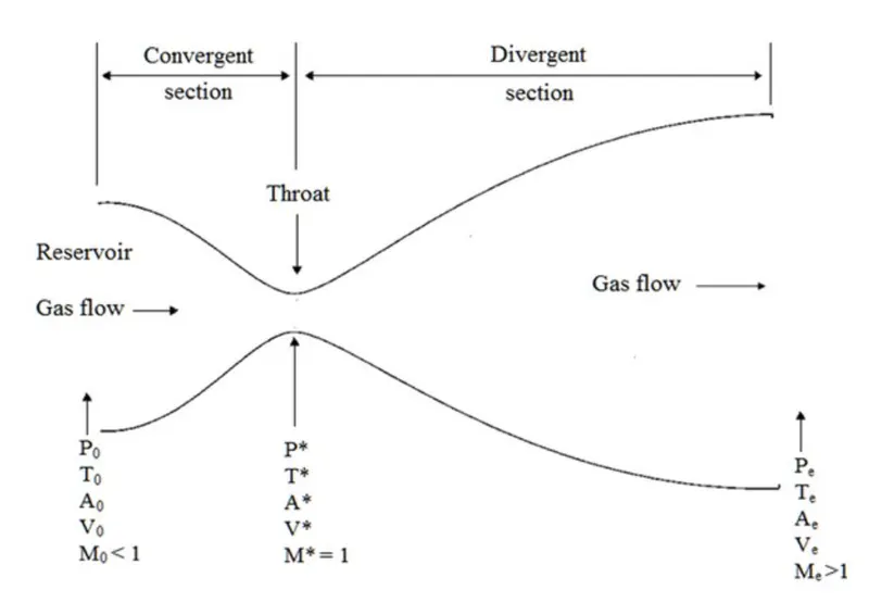
The symmetrical area function for the CD nozzle is given below:
`((A)/(Astar))^2=1+2.2(x-1.5)^2; 0<=x<=3`.
where `Astar`is the area at the throat of the nozzle and `x`is the distance along nozzle length. The non-dimensionalized form of the variables required for this problem are given below:
`x'=x/L; V'=V/a_o; t'=t/(L/a_o); rho'=rho/rho_o; T'=T/T_o; p'=p/p_o; A'=A/(Astar)`.
Governing Equations:
1. Non-Conservative Form: The non-conservative form of the governing equation which represents continuity, momentum and energy in terms of dimensionless variables is:
Continuity: `(delrho')/(delt')=-rho'((delV')/(delx'))-rho'V'((del(lnA'))/(delx'))-V'((delrho')/(delx'))`.
Momentum: `(delV')/(delt')=-V'((delV')/(delx'))-1/gamma[(delT')/(delx')+(T')/(rho').(delrho')/(delx')]`.
Energy: `(delT')/(delt')=-V'((delT')/(delx'))-(gamma-1)T'[(delV')/(delx')+V'((del(lnA'))/(delx'))]`.
The initial conditions as provided in the problem statement were:
1. `rho'(t=0)=1-0.3146x'`.
2. `T'(t=0)=1-0.2314x'`.
3. `V'(t=0)=(0.1+1.09x')sqrt(T'(t=0))`.
2. Conservative Form: The conservative form of the governing equation which represents continuity, momentum and energy in terms of dimensionless variables is:
Continuity: `(del(rho'A'))/(delt')+(del(rho'A'V'))/(delx')=0`.
Momentum: `(del(rho'A'V'))/(delt')+(del(rho'A'V'^2+(1/gamma)p'A'))/(delx')=1/gammap'(delA')/(delx')`.
Energy: `(del[rho'((T')/(gamma-1)+gamma/2V'^2)A'])/(delt')+(del[rho'((T')/(gamma-1)+gamma/2V'^2)V'A'+p'A'V'])/(delx')=0`.
In order to simplify these eqns. , we substitute the following terms, which include the solutions vectors `U_i`, the flux vectors `F_i`and the source term `J_2`.
`U_1=rho'A'`
`U_2=rho'A'V'`
`U_3=rho'[(T')/(gamma-1)+gamma/2V'^2]A'`
`F_1=rho'A'V'=U_2`
`F_2=rho'A'V'^2+1/gammap'A'=U_2^2/U_1+(gamma-1)/gamma[U_3-gamma/2(U_2^2/U_1)]`
`F_3=rho'((T')/(gamma-1)+gamma/2V'^2)V'A'+p'A'V'=gamma(U_2U_3)/U_1-(gamma(gamma-1))/2U_2^3/U_1^2`
`J_2=1/gammap'(delA')/(delx')`
After substituting these terms in the governing eqns., we have:
1. `(delU_1)/(delt')=-(delF_1)/(delx')`
2. `(delU_2)/(delt')=-(delF_2)/(delx')+J_2`
3. `(delU_3)/(delt')=-(delF_3)/(delx')`
The flow variables are calculated on numerical solution of the above terms as:
`rho'=U_1/(A')`
`V'=U_2/U_1`
`T'=(gamma-1)[U_3/U_1-gamma/2V'^2]`
`p'=rho'T'`
The initial conditions as provided in the problem statement are:
1. `rho'(t=0)`= 1.0 f or `0<=x'<0.5`
(1.0-0.366(x'-0.5)) f or `0.5<=x'<1.5`
0.634-0.3879(x'-1.5)) f or `1.5<=x'<3`
2. `T'(t=0)`= 1.0 f or `0<=x'<0.5`
1.0-0.167(x'-0.5)) f or `0.5<=x'<1.5`
(0.833-0.3507(x'-1.5)) f or `1.5<=x'<3`
3. `V'(t=0)=U_2/((rho'(t=0)A'))=0.59/((rho'(t=0)A')`
(considering a constant mass flow rate of `U_2=rho'A'V'=0.59`just for the initial condition)
MacCormack Method of Solving:
The MacCormack numerical scheme is a common method to solve flow eqns. It consists of 4 steps:
1. Predictor Step
2. Intermediate Solution Update
3. Corrector Step
4. Final Solution Update
In the predictor step, the spatial derivatives are calculated using the Forward Differencing Scheme(FDS). The time derivative from the governing eqns. obtained is recorded as `(delu)/(delt)_p`. Consider the continuity eqn. for the non-conservative form . From the predictor step, we obtain:
`((delrho_i)/(delt))_P=-rho'_i[([V'_(i+1)-V_i'])/(trianglex')]-rho'_iV'_i[(ln(A'_(i+1))-ln(A'_i))/(trianglex')]-V'_i([rho'_(i+1)-rho'_i]/(trianglex'))`
During the intermediate solution update, the variable is updated based on the time derivative obtained from the predictor step as:
`rho_(i,P)^(t+trianglet)=rho'_i+((delrho'_i)/(delt'))_Ptrianglet`
Using these updated values, the governing equations are solved again using BDS in space in the corrector step. The time derivative obtained during the corrector step is stored as `((delu)/(delt))_C`.
`((delrho_i)/(delt))_C=-rho'_(i,P)[([V'_(i,P)-V_(i-1,P)'])/(trianglex')]-rho'_(i,P)V'_(i,P)[(ln(A'_(i,P))-ln(A'_(i-1,P)))/(trianglex')]-V'_(i,P)([rho'_(i,P)-rho'_(i-1,P)]/(trianglex'))`
For the final solution update, we use the averages of the time derivatives obtained using the predictor and corrector steps. Since, we're usinng FDS in predictor step and BDS in corrector step, the average of the time-derivative for the final update, overall scheme becomes a second order numerical scheme.
`((delrho)/(delt))_(av)=1/2[((delrho)/(delt))_P+((delrho)/(delt))_C]`
`rho_(i)^(t+trianglet)=rho_i^t+((delrho)/(delt))_(av)trianglet`
Main MATLAB Code:
clear all
close all
clc

% Initializing the domain
L=3;
nx=61;
x=linspace(0,L,nx);
dx=x(2)-x(1);
C=0.5;
nt=1400;
gamma=1.4;

% Nozzle area profile
A=1+2.2*(x-1.5).^2;

% Computing the flow variable through conservative & non-conservative form
[rho1,V1,T1,p1,M1,m1,rho_t1,V_t1,p_t1,T_t1,M_t1,residual1]=nonconservative(x,dx,A,C,nt,gamma);
[rho2,V2,T2,p2,M2,m2,rho_t2,V_t2,p_t2,T_t2,M_t2,residual2]=conservative(x,dx,A,C,nt,gamma);

% Plotting the results
figure(1)
subplot(4,1,1)
plot(x,M1)
grid on;
ylim([0 4.5]);
yticks(0:1.5:4.5);
ylabel('Mach Number')
title('Flow parameter(non-conservative form of governing eqn.)')
subplot(4,1,2)
plot(x,p1)
grid on;
yticks(0:0.2:1);
ylabel('Pressure Ratio')
subplot(4,1,3)
plot(x,rho1)
grid on;
yticks(0:0.2:1);
ylabel('Density Ratio')
subplot(4,1,4)
plot(x,T1)
grid on;
ylim([0 1]);
yticks(0:0.2:1);
ylabel('Temperature Ratio')
xlabel('X/L')

figure(2)
subplot(4,1,1)
plot(x,M2)
grid on;
ylim([0 4.5]);
yticks(0:1.5:4.5);
ylabel('Mach Number')
title('Flow parameter(conservative form of governing eqn.)')
subplot(4,1,2)
plot(x,p2)
grid on;
yticks(0:0.2:1);
ylabel('Pressure Ratio')
subplot(4,1,3)
plot(x,rho2)
grid on;
yticks(0:0.2:1);
ylabel('Density Ratio')
subplot(4,1,4)
plot(x,T2)
grid on;
ylim([0 1]);
yticks(0:0.2:1);
ylabel('Temperature Ratio')
xlabel('X/L')

figure(3)
subplot(4,1,1)
plot(1:nt,rho_t1)
hold on;
plot(1:nt,rho_t2)
grid on;
ylim([0 1]);
yticks(0:0.2:1);
ylabel('rho/rho_0')
title('Flow parameter variation with time at the nozzle throat');
legend('Non-conservative','Conservative');
subplot(4,1,2)
plot(1:nt,T_t1)
hold on;
plot(1:nt,T_t2)
grid on;
yticks(0:0.2:1);
ylabel('T/T_0')
legend('Non-conservative','Conservative');
subplot(4,1,3)
plot(1:nt,p_t1)
hold on;
plot(1:nt,p_t2)
grid on;
yticks(0:0.2:1);
ylabel('p/p_0')
legend('Non-conservative','Conservative')
subplot(4,1,4)
plot(1:nt,M_t1)
hold on;
plot(1:nt,M_t2)
grid on;
yticks(0:0.2:2);
ylabel('Mach No.')
xlabel('Time Steps')
legend('Non-conservative','Conservative')

figure(4)
subplot(2,1,1)
plot(1:nt,residual1)
grid on;
xlabel('Time Steps')
ylabel('Residuals')
legend('|drho/dt|_{av}','|dV/dt|_{av}','|dT/dt_{av}')
title('Residuals: Non-conservative form')
subplot(2,1,2)
plot(1:nt,residual2)
grid on;
xlabel('Time Steps')
ylabel('Residuals')
yticks(0:0.5:4);
legend('|dU_1/dt_{av}','|dU_2/dt|_{av}','|dU_3/dt|_{av}')
title('Residuals: Conservative form')

figure(5)
hold on;
grid on;
plot(x,m1(50,:),'-x')
plot(x,m1(100,:),'-d')
plot(x,m1(150,:),'-s')
plot(x,m1(200,:),'-*')
plot(x,m1(700,:),'-o')
xlabel('X/L')
ylabel('rhoAV/rho_0A_0V_0')
legend('t=50/t','t-=100/t','t=150/t','t=200/t','t=700/t')
title('Variation of non-dimensional mass flow rate(Non-conservative form)')

figure(6)
hold on;
grid on;
plot(x,m2(100,:),'-x')
plot(x,m2(150,:),'-d')
plot(x,m2(200,:),'-*')
plot(x,m2(700,:),'-o')
xlabel('X/L')
ylabel('rhoAV/rho_0A_0V_0')
legend('t=100/t','t-=150/t','t=200/t','t=700/t')
title('Variation of non-dimensional mass flow rate(Conservative form)')

figure(7)
hold on;
grid on;
plot(x,m1(end,:),'LineWidth',3)
plot(x,m2(end,:),'LineWidth',3)
plot(x,0.579*ones(length(x),1),'--k')
xlabel('X/L')
ylabel('rhoAV/rho_0A_0V_0')
legend('Non-conservative','Conservative','Exact')
title('Variation of non-dimensional mass flow rate(Steady State)')
Function for Conservative Form of Governing Equation:
% Solver for conservative form of governing equation

function [rho,V,T,p,M,m,rho_t,V_t,p_t,T_t,M_t,residual]=conservative(x,dx,A,C,nt,gamma)
% Initial conditions
throat=find(A==1);
rho_0=zeros(1,length(x));
T_0=rho_0;
V_0=T_0;
for i=1:length(x)
    if x(i)>=0 && x(i)<0.5
        rho_0(i)=1;
         T_0(i)=1;
    elseif x(i)>=0.5 && x(i)<1.5
        rho_0(i)=1-0.366*(x(i)-0.5);
        T_0(i)=1-0.167*(x(i)-0.5);
    elseif x(i)>=1.5 && x(i)<=3
        rho_0(i)=0.634-0.3879*(x(i)-1.5);
        T_0(i)=0.833-0.3507*(x(i)-1.5);
    end
    V_0(i)=0.59/(rho_0(i)*A(i));
end

rho=rho_0;
T=T_0;
V=V_0;
m=zeros(nt,length(x));
U1=rho.*A;
U2=rho.*A.*V;
U3=rho.*(T./(gamma-1)+(0.5*gamma)*(V.^2)).*A;
rho_t=zeros(nt,1);
T_t=rho_t;
V_t=T_t;
p_t=V_t;
M_t=p_t;
residual=zeros(nt,3);
for k=1:nt
    U1_old=U1;
    U2_old=U2;
    U3_old=U3;
    dt=min(C*dx./(T.^0.5+V));
    F1=U2;
    F2=(U2.^2)./U1+(gamma-1)/(gamma)*(U3-0.5*gamma*(U2.^2)./U1);
    F3=gamma*U2.*U3./U1-0.5*gamma*(gamma-1)*(U2.^3)./(U1.^2);
    % Predictor Loop
    for i=2:length(x)-1
        dF1dx=(F1(i+1)-F1(i))/dx;
        dF2dx=(F2(i+1)-F2(i))/dx;
        dF3dx=(F3(i+1)-F3(i))/dx;
        dAdx=(A(i+1)-A(i))/dx;
        J2=(1/gamma)*rho(i)*T(i)*dAdx;

        dU1dt_p(i)=-dF1dx;
        dU2dt_p(i)=-dF2dx+J2;
        dU3dt_p(i)=-dF3dx;

        % Intermediate update
        U1(i)=U1(i)+dU1dt_p(i)*dt;
        U2(i)=U2(i)+dU2dt_p(i)*dt;
        U3(i)=U3(i)+dU3dt_p(i)*dt;
    end
    rho=U1./A;
    V=U2./U1;
    T=(gamma-1)*((U3./U1)-0.5*gamma*V.^2);
    F1=U2;
    F2=((U2.^2)./U1)+(((gamma-1)/gamma)*(U3-((0.5*gamma)*(U2.^2)./U1)));
    F3=(gamma*((U2.*U3)./U1))-((0.5*gamma*(gamma-1))*((U2.^3)./U1.^2));
    % Corrector Loop
    for i=2:length(x)-1
        dF1dx=(F1(i)-F1(i-1))/dx;
        dF2dx=(F2(i)-F2(i-1))/dx;
        dF3dx=(F3(i)-F3(i-1))/dx;
        dAdx=(A(i)-A(i-1))/dx;
        J2=(1/gamma)*rho(i)*T(i)*dAdx;

        dU1dt_c(i)=-dF1dx;
        dU2dt_c(i)=-dF2dx+J2;
        dU3dt_c(i)=-dF3dx;
    end

    % Average of predictor and corrector step
    dU1dt=0.5*(dU1dt_p+dU1dt_c);
    dU2dt=0.5*(dU2dt_p+dU2dt_c);
    dU3dt=0.5*(dU3dt_p+dU3dt_c);
    residual(k,1)=max(abs(dU1dt));
    residual(k,2)=max(abs(dU2dt));
    residual(k,3)=max(abs(dU3dt));

    % Final solution update
    for i=2:length(x)-1
        U1(i)=U1_old(i)+dU1dt(i)*dt;
        U2(i)=U2_old(i)+dU2dt(i)*dt;
        U3(i)=U3_old(i)+dU3dt(i)*dt;
    end

    % Boundary Conditions
    U1(1)=rho(1)*A(1);
    U1(end)=2*U1(end-1)-U1(end-2);
    U2(1)=2*U2(2)-U2(3);
    U2(end)=2*U2(end-1)-U2(end-2);
    U3(1)=U1(1)*((T(1)/(gamma-1))+0.5*gamma*V(1)^2);
    U3(end)=2*U3(end-1)-U3(end-2);
    rho=U1./A;
    V=U2./U1;
    T=(gamma-1)*((U3./U1)-((0.5*gamma)*V.^2));
    M=V./(T.^0.5);
    p=rho.*T;
    m(k,:)=rho.*A.*V;
    rho_t(k)=rho(throat);
    V_t(k)=V(throat);
    T_t(k)=T(throat);
    p_t(k)=p(throat);
    M_t(k)=M(throat);
end
end
Function for Non-Conservative Form of Governing Equation:
% Solver for non-conservative form of governing equation

function [rho,V,T,p,M,m,rho_t,V_t,p_t,T_t,M_t,residual]=nonconservative(x,dx,A,C,nt,gamma)
% Initial Conditions
rho_1=1-0.3146*x;
T_1=1-0.2314*x;
V_1=(0.1+1.09*x).*T_1.^0.5;
throat=find(A==1);
rho=rho_1;
T=T_1;
V=V_1;
m=zeros(nt,length(x));
rho_t=zeros(nt,1);
T_t=rho_t;
V_t=T_t;
p_t=V_t;
M_t=p_t;
residual=zeros(nt,3);
for k=1:nt
    rho_old=rho;
    T_old=T;
    V_old=V;
    dt=min(C*dx./(T.^0.5+V));
    % Predictor Loop
    for i=2:length(x)-1
        dVdx=(V(i+1)-V(i))/dx;
        dlogAdx=(log(A(i+1))-log(A(i)))/dx;
        drhodx=(rho(i+1)-rho(i))/dx;
        dTdx=(T(i+1)-T(i))/dx;

        drhodt_p(i)=-rho(i)*dVdx-rho(i)*V(i)*dlogAdx-V(i)*drhodx;
        dVdt_p(i)=-V(i)*dVdx-(1/gamma)*(dTdx+((T(i)/rho(i))*drhodx));
        dTdt_p(i)=-V(i)*dTdx-(gamma-1)*T(i)*(dVdx+V(i)*dlogAdx);

        % Intermediate update
        rho(i)=rho(i)+drhodt_p(i)*dt;
        V(i)=V(i)+dVdt_p(i)*dt;
        T(i)=T(i)+dTdt_p(i)*dt;
    end

    % Corrector Loop
    for i=2:length(x)-1
        dVdx=(V(i)-V(i-1))/dx;
        dlogAdx=(log(A(i))-log(A(i-1)))/dx;
        drhodx=(rho(i)-rho(i-1))/dx;
        dTdx=(T(i)-T(i-1))/dx;

        drhodt_c(i)=-rho(i)*dVdx-rho(i)*V(i)*dlogAdx-V(i)*drhodx;
        dVdt_c(i)=-V(i)*dVdx-((1/gamma)*(dTdx+((T(i)/rho(i))*drhodx)));
        dTdt_c(i)=-V(i)*dTdx-(gamma-1)*T(i)*(dVdx+V(i)*dlogAdx);
    end

    % Average of predictor and corrector step
    drhodt=0.5*(drhodt_p+drhodt_c);
    dVdt=0.5*(dVdt_p+dVdt_c);
    dTdt=0.5*(dTdt_p+dTdt_c);
    residual(k,1)=max(abs(drhodt));
    residual(k,2)=max(abs(dVdt));
    residual(k,3)=max(abs(dTdt));

    % Final solution update
    for i=2:length(x)-1
        rho(i)=rho_old(i)+drhodt(i)*dt;
        V(i)=V_old(i)+dVdt(i)*dt;
        T(i)=T_old(i)+dTdt(i)*dt;
    end

    % Boundary Conditions
    rho(end)=2*rho(end-1)-rho(end-2);
    V(1)=2*V(2)-V(3);
    V(end)=2*V(end-1)-V(end-2);
    T(end)=2*T(end-1)-T(end-2);
    M=V./(T.^0.5);
    p=rho.*T;
    m(k,:)=rho.*A.*V;
    rho_t(k)=rho(throat);
    V_t(k)=V(throat);
    T_t(k)=T(throat);
    p_t(k)=p(throat);
    M_t(k)=M(throat);
end
end
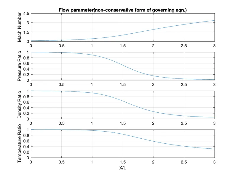
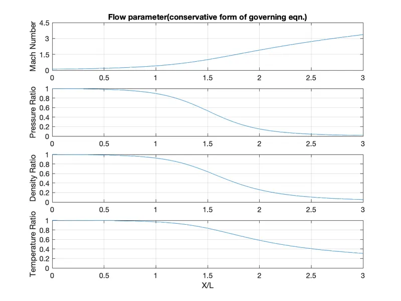
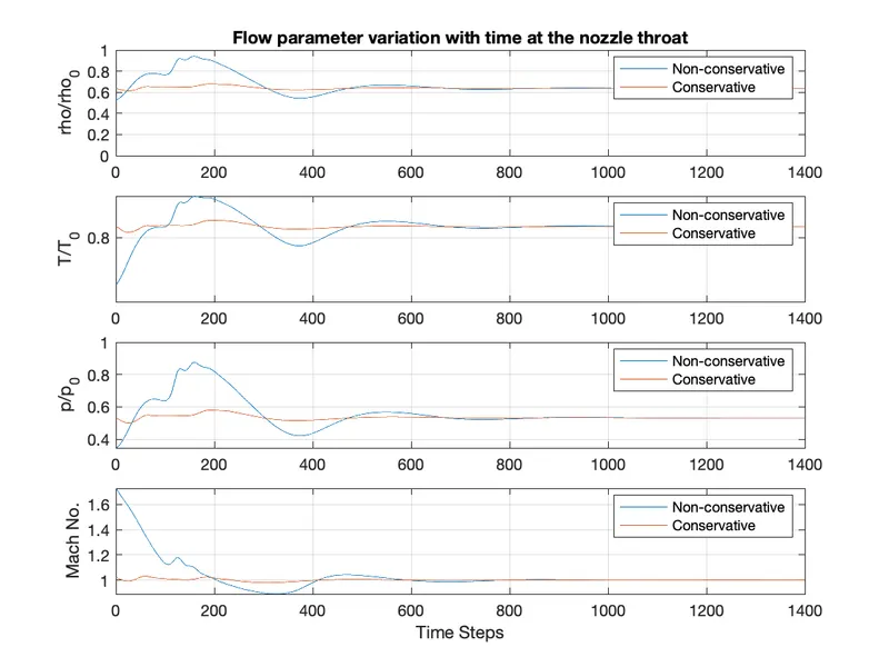
Output Graphs:
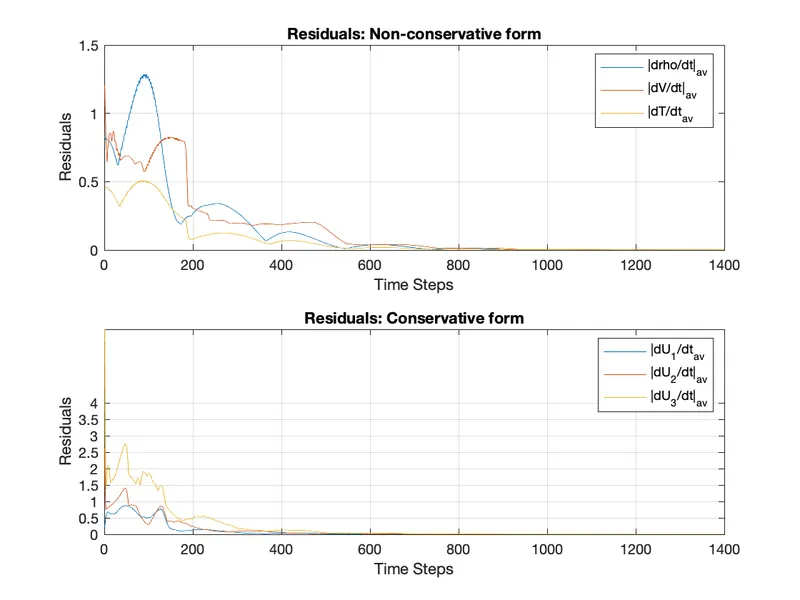
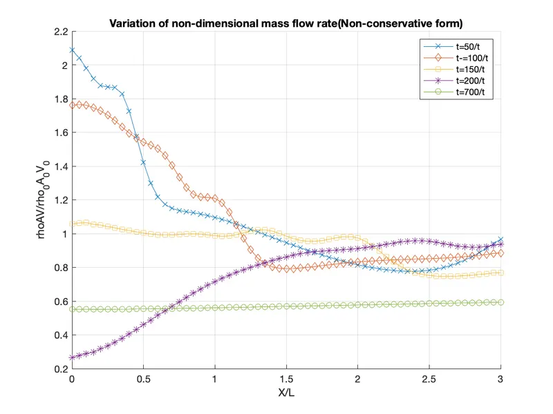
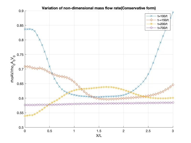
Mass Flow At nx=61:
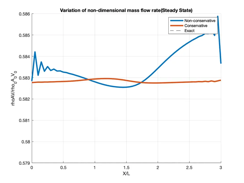
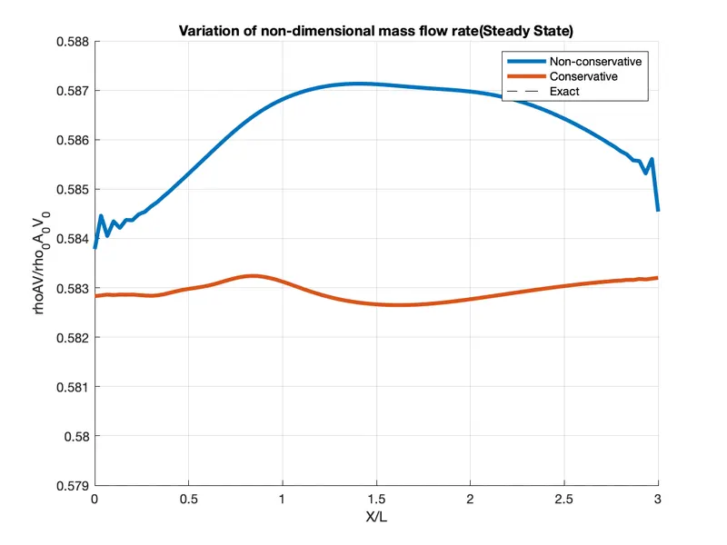
Mass Flow At nx=91:
Results and Conclusion:
1. For comparing the conservative and non-conservative form, the values of the flow variables at the throat of the nozzle are plotted at each time step. It is observed that at smaller time steps, the behaviour of non-conservative form shows unstable results, but with increase in time step, the difference in conservative and non-conservative approach diminishes.
2. If we notice the residuals of both the approaches, the conservative form converges to a steady state faster than the non-conservative form.
3. There is an appreciable difference in how mass flow rate varies with time step, but it can be observed that at the time step `700trianglet`, the mass flow becomes constant. Moreover, the conservative form produces an almost constant mass flow rate, but the non-conservative approach gives a highly fluctuating mass flow rate.
4. On varying the grid size, it is noted that the conservative form almost maintains its consistency, but the non-conservative form tends to become stable on inceasing grid size.
5. Thus, MacCormack Method provides quite stable and close-to-exact solutions, hence it is widely used to solve various flow problems.