Week 11 - Simulation of Flow through a pipe in OpenFoam
Objectives: 1. To simulate a 2D incompressible flow through a cylinder pipe in OPENFOAM.
2. Compare the velocity profile and maximum shear stress for the fully developed flow along with the pressure drop with the Hagen-Poiseuille's equation.
3. To make arrangements for the saving of computational resources and time by reducing the model geometrically.
Problem Definition: Here, we're considering a circular pipe of diameter 20mm and length 2.7m through which the flowing fluid is water with density of 1000 `(kg)/m^3`and dynamic viscosity of 0.00089 Pa.s. As per the calculations, to keep the flow laminar, the average velocity of the flow has to be taken as 0.0935 m/s and thus the Reynold's number, `R_e`=2100. For a circular pipe, the flow becomes turbulent after when Reynold's number becomes greater than 4000 and in-between 2300 and 4000, the flow remains in the transition state.
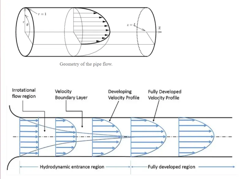
At the entrance, the flow is said to be in hydrodynamic entrance region where the velocity profile gradually takes the shape of a parabola from a straight line. As soon as the parabolic velocity profile becomes steady, the flow is said to be in its fully developed state. Usually, Hagen-Poiseuille's equation is applicable for fully developed flow which helps us to calculate the pressure loss. For a circular pipe, we can calculate the average and maximum velocity, maximum shear stress and pressure loss analytically which is shown below:
`v_(avg)=(muR_e)/(rhoD_h)`
`v_(max)=2v_(avg)`
`tau_(max)=(2muv)/r_h`
Hagen-Poiseuille's Equation:
`P_(loss)=(32mu(L-L_e)v_(avg))/(D_h^2)`
wherein `v_(avg)`= Average Velocity, `v_(max)`= Maximum Velocity, `tau_(max)`= Maximum Shear Stress, `mu`= Dynamic Viscosity, `r_h`= Hydraulic Radius of Pipe, `D_h`= Hydraulic Diameter of Pipe, `P_(loss)`= Pressure Loss, `L_e`= Entrance Length=`0.06R_eD_h`(for laminar flow through a circular pipe)
Governing Equations: Here, we will try to solve the Navier-Stokes Equation and the Continuity Equation.
Continuity Equation:
`(delrho)/(delt)+(delrhou)/(delx)+(delrhov)/(dely)+(delrhow)/(delz)=0`
Momentum Equations:
1. `(delrhou)/(delt)+(delrhou^2)/(delx)+(delrhouv)/(dely)+(delrhouw)/(delz)=-(delp)/(delx)+1/(R_er)[(del tau_(x x))/(delx)+(del tau_(xy))/(dely)+(del tau_(xz))/(delz)]`
2. `(delrhov)/(delt)+(delrhouv)/(delx)+(delrhov^2)/(dely)+(delrhovw)/(delz)=-(delp)/(dely)+1/(R_er)[(del tau_(x x))/(delx)+(del tau_(xy))/(dely)+(del tau_(xz))/(delz)]`
3. `(delrhow)/(delt)+(delrhouw)/(delx)+(delrhovw)/(dely)+(delrhow^2)/(delz)=-(delp)/(delz)+1/(R_er)[(del tau_(x x))/(delx)+(del tau_(xy))/(dely)+(del tau_(xz))/(delz)]`
* We will use the icoFoam solver of OPENFOAM to solve the incompressible problem and the above mentioned equation.
Main MATLAB Code:
% ***************************** %
%% OpenFOAM Pipe Flow Challenge
%% Author: Saikiran.P
%% Date: 15 June 2021
% ***************************** %

clear all
close all
clc

%% Problem Initialization
%  Material: Water at 25 deg C inside
%  Outside: Ambient Condition
Re=2100;    % Reynolds Number
rho=1000;   % Density at 25 deg C: Unit: kg/m^3
mu=0.89e-3; % 0.00089; % nu*rho; % Dynamic Viscosity at 25 deg C: Unit: Pa.s
nu=mu/rho;  % Kinematic Viscosity at 25 deg C: Unit: m^2/s

D=0.02;          % Dia of pipe in meters
A_c=(pi/4)*D^2;  % Cross Sectional Area
p=pi*D;          % Wetted Perimeter
D_h=4*A_c/p;     % Hydraulic Dia of Pipe
r_h=D_h/2;       % Hydraulic Radius of Pipe
v_avg=(Re*mu)/(rho*D_h); % Average Velocity
v_max=2*v_avg;           % Fully Developed V max
tau_max=2*mu*v_max/r_h;

if Re<2300
    L_e=0.06*Re*D_h;        % From Cengel Fluid Dynamics Book
elseif Re==2300             % From Cengel Fluid Dynamics Book
    L_e=115*D_h;
elseif Re>4000
    L_e=1.359*D_h*Re^(1/4); % From Bhatti & Shah and Zhi-Qing
    % L_e=10*D_h-----> Approximately calculated as:
end

L=L_e+0.18;                 % Meters-----> Length of Pipe

%% Pressure Loss
% Daracy Friction Factory----> for Laminar Circular Pipe Flow
f=65/Re;

% Hagen- Poiseuille's equation:

P=(32*mu*(L-L_e)*v_avg)/(D^2);
g=9.81;
h_loss=P/(rho*g); % Head Loss
P_kinematicPress=P/rho;
theta=3;          % 3 degree wedge angle
r=r_h;

%% Print Out
sys(r,L,theta)
Function:
function sys(r,L,theta)

%% Creating blockmeshdict file
%% Opening Part
h1='/*--------------------------------*- C++ -*--------------------------------*';
h2='  =========                  |;
h3='  \       / F ield           | OpenFOAM: The Open Source CFD Toolbox';
h4='   \     /  O peration       | Website: https://openfoam.org';
h5='    \   /   A nd             | Version: 8';
h6='     \ /    M anipulation    | Date: 25 Oct 2020';
h7='                             | Author: Saikiran.P';
h8='*--------------------------------------------------------------------------*/';
h9='FoamFile';
h10='{';
h11='     version      2.0;';
h12='     format       ascii;';
h13='     class        dictionary;';
h14='     object       blockMeshDict;';
h15='}';
h16='// * * * * * * * * * * * * * * * * * * * * * * * * * * * * * * * * * * * * //';
f1=fopen=('blockMeshDict.txt','wt');

fprintf(f1,'%sn',h1);
fprintf(f1,'%sn',h2);
fprintf(f1,'%sn',h3);
fprintf(f1,'%sn',h4);
fprintf(f1,'%sn',h5);
fprintf(f1,'%sn',h6);
fprintf(f1,'%sn',h7);
fprintf(f1,'%sn',h8);
fprintf(f1,'%sn',h9);
fprintf(f1,'%sn',h10);
fprintf(f1,'%sn',h11);
fprintf(f1,'%sn',h12);
fprintf(f1,'%sn',h13);
fprintf(f1,'%sn',h14);
fprintf(f1,'%sn',h15);
fprintf(f1,'%sn',h16);

%% Vertices

v0=[0 0 0];
v1=[0 r*cosd(theta/2) r*sind(theta/2)];
v2=[0 r*cosd(theta/2) -r*sind(theta/2)];
v3=[L 0 0];
v4=[L r*cosd(theta/2) r*sind(theta/2)];
v5=[L r*cosd(theta/2) -r*sind(theta/2)];
mid1=[0 r 0];
mid2=[L r 0];

%% Write Vertices
h17='convertToMeters 1;';
fprintf(f1,'%sn',h17);

h18='vertices';
fprintf(f1,'%sn',h18);
h19='(';
fprintf(f1,'%sn',h19);
fprintf(f1,'t(%d %d %d)n',v0);
fprintf(f1,'t(%d %d %d)n',v1);
fprintf(f1,'t(%d %d %d)n',v2);
fprintf(f1,'t(%d %d %d)n',v3);
fprintf(f1,'t(%d %d %d)n',v4);
fprintf(f1,'t(%d %d %d)n',v5);
h20=');';
fprintf(f1,'%sn',h20);

%% Write Blocks
h21='blocks';
h22='(';
h23='     hex(0 3 4 1 0 3 5 2) (200 50 1) simpleGrading (1 0.2 1)';
h24=');';
fprintf(f1,'%sn',h21);
fprintf(f1,'%sn',h22);
fprintf(f1,'%sn',h23);
fprintf(f1,'%sn',h24);

%% Write Edges
h25='edges';
h26='(';
h27='   arc 2 1';
h28='   arc 5 4';
h29=');';

fprintf(f1,'%sn',h25);
fprintf(f1,'%sn',h26);
fprintf(f1,'%s (%d %d %d)n',h27,0,r,0);
fprintf(f1,'%s (%d %d %d)n',h28,L,r,0);
fprintf(f1,'%sn',h29);

%% Write Boundary
inlet=[0 1 2 0];
outlet=3 5 4 3];
surface=[2 1 4 5];
axis=[0 3 3 0];
front=[1 0 3 4];
back=[0 2 5 3];

fprintf(f1,'%sn','boundary');
fprintf(f1,'%sn','(');
% Inlet Patch
fprintf(f1,'t%sn','inlet');
fprintf(f1,'t%sn','{');
fprintf(f1,'tt%sn','type patch');
fprintf(f1,'tt%sn','faces');
fprintf(f1,'tt%sn','(');
fprintf(f1,'ttt(%d %d %d)n',inlet);
fprintf(f1,'tt%sn',');');
fprintf(f1,'t%sn','}');

% Outlet Patch
fprintf(f1,'t%sn','outlet');
fprintf(f1,'t%sn','{');
fprintf(f1,'tt%sn','type patch');
fprintf(f1,'tt%sn','faces');
fprintf(f1,'tt%sn','(');
fprintf(f1,'ttt(%d %d %d)n',outlet);
fprintf(f1,'tt%sn',');');
fprintf(f1,'t%sn','}');

% Surface
fprintf(f1,'t%sn','surface');
fprintf(f1,'t%sn','{');
fprintf(f1,'tt%sn','type wall');
fprintf(f1,'tt%sn','faces');
fprintf(f1,'tt%sn','(');
fprintf(f1,'ttt(%d %d %d)n',surface);
fprintf(f1,'tt%sn',');');
fprintf(f1,'t%sn','}');

% Axis
fprintf(f1,'t%sn','axis');
fprintf(f1,'t%sn','{');
fprintf(f1,'tt%sn','type empty');
fprintf(f1,'tt%sn','faces');
fprintf(f1,'tt%sn','(');
fprintf(f1,'ttt(%d %d %d)n',axis);
fprintf(f1,'tt%sn',');');
fprintf(f1,'t%sn','}');

% Front
fprintf(f1,'t%sn','front');
fprintf(f1,'t%sn','{');
fprintf(f1,'tt%sn','type wedge');
fprintf(f1,'tt%sn','faces');
fprintf(f1,'tt%sn','(');
fprintf(f1,'ttt(%d %d %d)n',front);
fprintf(f1,'tt%sn',');');
fprintf(f1,'t%sn','}');

% Back
fprintf(f1,'t%sn','back');
fprintf(f1,'t%sn','{');
fprintf(f1,'tt%sn','type wedge');
fprintf(f1,'tt%sn','faces');
fprintf(f1,'tt%sn','(');
fprintf(f1,'ttt(%d %d %d)n',back);
fprintf(f1,'tt%sn',');');
fprintf(f1,'t%sn','}');
fprintf(f1,'%sn',');');

fprintf(f1,'%sn','mergePatchPairs');
fprintf(f1,'%sn','(');
fprintf(f1,'%sn',');');
fprintf(f1,'%sn','// **************************************************** //');

end
OPENFOAM Files:
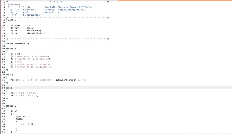
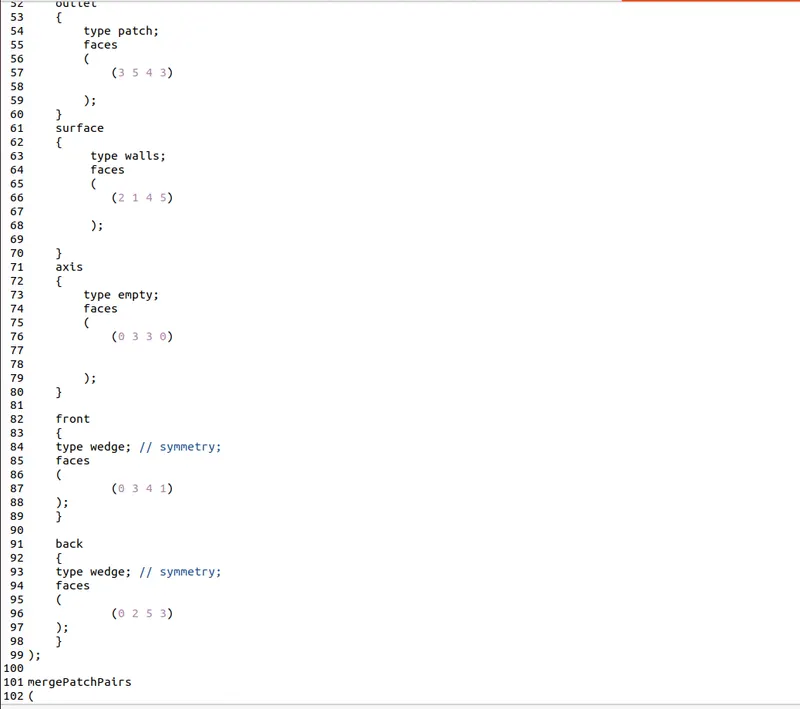
1. blockMeshDict:

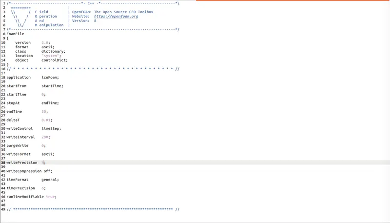
2. controlDict:
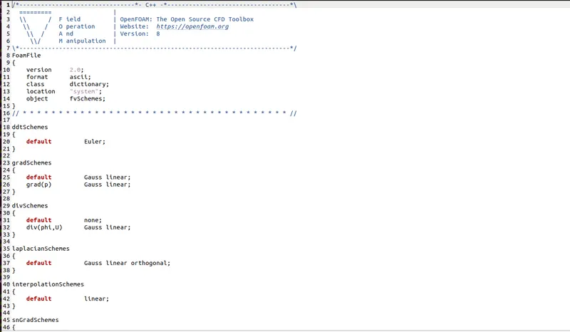
3. fvSchemes:

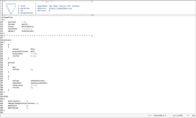
4. fvSolution:

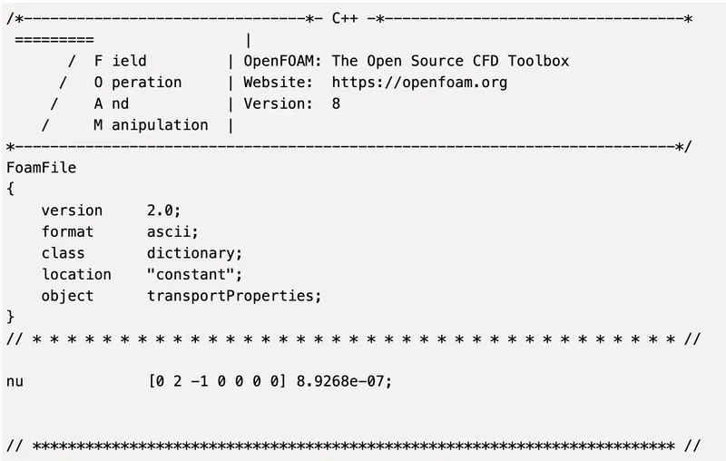
5. transportProperties:
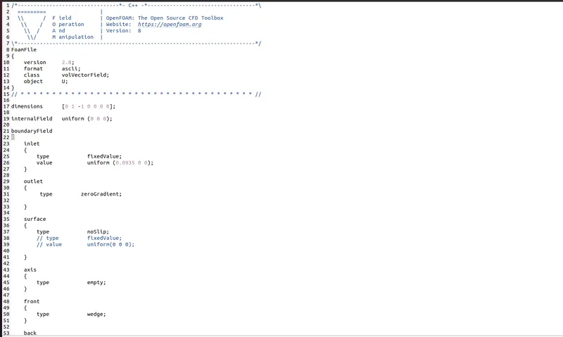
6. U(Velocity):

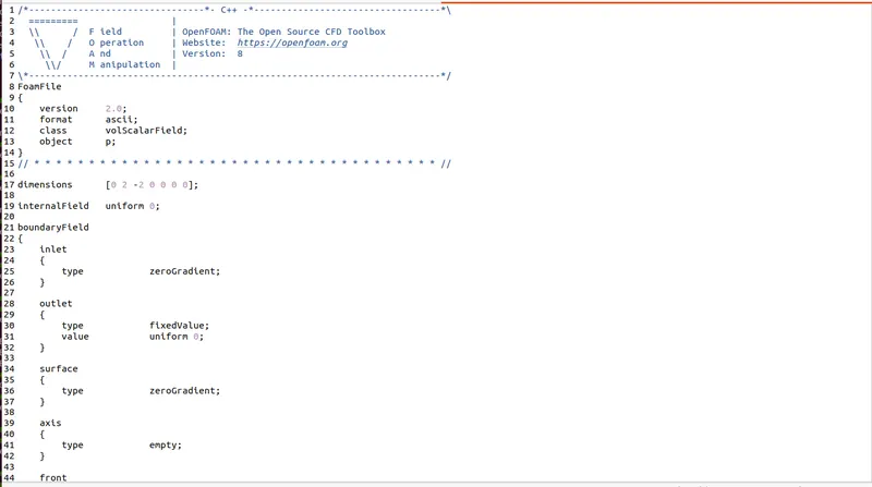
7. p(Pressure):

Algorithm: 1. In the first step, we have defined the geometry parameters and then passed the radius, length of pipe and wedge angle to the sys() function which basically printed the blockMeshDict file.
2. We have set the file structure of the OPENFOAM for the icoFoam solver.
3. Afterwards, we have typed the following keys: blockMesh--->checkMesh--->icoFoam.
4. Post-processing was accomplished using paraView.
Output Graphs:
For Wedge Angle 3 Degrees:
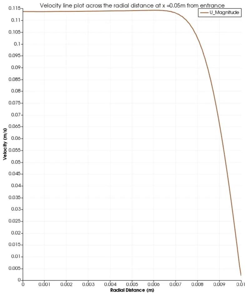
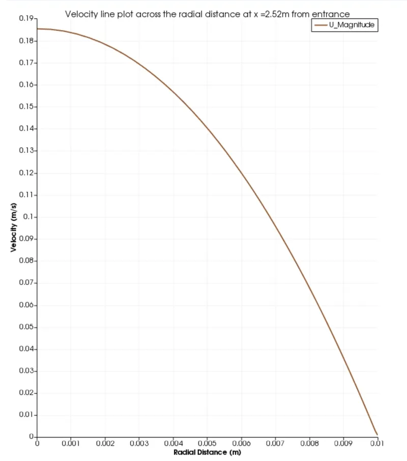
1. Velocity Plot:
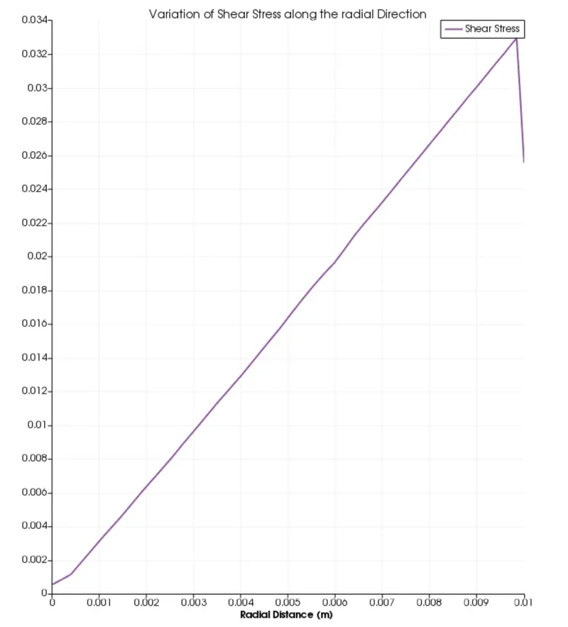
2. Maximum Shear Stress Plot:
Results and Discussion:
| Maximum Velocity(m/s) | Pressure Loss(Pa) | Maximum Shear Stress(Pa) | |
| Numerical Results | 0.1854 | 0.00121065 | 0.03279 |
| Theoretical Results | 0.1869 | 0.0012 | 0.0333 |
We can observe that the results are similar to the theoretical results. The velocity profile we obtained is parabolic in shape which basically signifies that the flow is fully developed. An example for developing velocity flow is given below: