Week 3.5 - Deriving 4th order approximation of a 2nd order derivative using Taylor Table method

Aim: To derive and write a program for fourth order approximation of a second order derivative in MATLAB by the following methods:

1. Central Difference

2. Skewed Right Sided Difference

3. Skewed Left Sided Difference

Objective: 1. To evaluate the second order derivative of the function `f(x)=exp(x)*cos(x)`using above mentioned order of approximations.

2. To plot and compare the values and errors of the 3 methods derived.

Theory and Derivations: During the solving of a CFD problem, we may come across a partial derivative equation which consists of second order derivative. Due to the complexity of the equation, we may have to choose numerical approach rather that analytical. When dealing with the former, we try to make the margin of error as low as possible. As the order of approximation gets higher, higher accuracy is obtained. Hence, we are going to derive the three methods of approximation for an analytical function. The methods are seen below:
1. Central Difference: Here, the nodes selected are symmetrical i.e. data is taken from both sides of point of focus. Using Taylor's method, we get:

`(delta^2f)/(deltax^2)=af(i-2)+bf(i-1)+cf(i)+df(i+1)+ef(i+2)`

Here, there are 2 nodes taken from both sides of point of focus i.e. f(i).

To select the number of nodes in consideration, we use following expression:

N=p+q-1 for central differencing

N=p+q for skewed differencing

Here, N is no. of nodes, p is order of derivative and q is order of approximation.

Taylor's Table for Central Difference:

	f(x)	dxf'(x)	dx^2f''(x)	dx^3f'''(x)	dx^4f''''(x)	dx^5f'''''(x)
af(i-2)	a	-2a	4a/2	-8a/6	16a/24	-32a/120
bf(i-1)	b	-b	b/2	-b/6	b/24	-b/120
cf(i)	c	0	0	0	0	0
df(i+1)	d	d	d/2	d/6	d/24	d/120
ef(i+2)	e	2e	4e/2	8e/6	16e/24	32e/120
af(i-2)+bf(i-1)+cf(i)+df(i+1)+ef(i+2)	0	0	1	0	0	?

The table transforms into matrix of type AX=B.

`[[1,1,1,1,1],[-2,-1,0,1,2],[4/2,1/2,0,1/2,4/2],[1,2,3,4,5],[-8/6,1/6,0,1/6,8/6],[16/24,1/24,0,1/24,16/24]]*[[a],[b],[c],[d],[e]]=[[0],[0],[1],[0],[0]]`

On further solving, we get the values of the unknown.

i.e. Values, a=-0.0833; b=1.3333; c=-2.5000; d=1.3333; e=-0.0833.

These coefficients will be further used in the code to get the value of the derivative.

2. Skewed Right Sided Difference: When the data points of the left nodes are not available(at initial boundary conditions), then we have to rely on the available data set.

`(delta^2f)/(delta x^2)=af(i)+bf(i+1)+cf(i+2)+df(i+3)+ef(i+4)+ff(i+5)`

Taylor's Table for Skewed Right Sided Difference:

	f(x)	dxf'(x)	dx^2f''(x)	dx^3f'''(x)	dx^4f''''(x)	dx^5f'''''(x)
af(i)	a	0	0	0	0	0
bf(i+1)	b	b	b/2	b/6	b/24	b/120
cf(i+2)	c	2c	4c/2	8c/6	16c/24	32c/120
df(i+3)	d	3d	9d/2	27d/6	81d/24	243d/120
ef(i+4)	e	4e	16e/2	64e/6	256e/24	1024e/120
ff(i+5)	f	5f	25f/2	125f/6	625f/24	3125f/120
af(i)+bf(i+1)+cf(i+2) +df(i+3)+ef(i+4)+ff(i+5)	0	0	1	0	0	0

This table transforms into a matrix of type AX=B.

`[[1,1,1,1,1,1],[0,1,2,3,4,5],[0,1/2,2,9/2,16/2,25/2],[0,1/6,8/6,27/6,64/6,125/6],[0,1/24,16/24,81/24,256/24,625/24],[0,1/120,32/120,243/120,1024/120,3125/120]]*[[a],[b],[c],[d],[e],[f]]=[[0],[0],[1],[0],[0],[0]]`

On further solving, we get the values of unknown.

i.e. Values, a=3.7500; b=-12.8333; c=17.8333; d=-13.0000; e=5.0833; f=-0.8333.

These coefficients will be further used in the code to get the value of the derivative.

3. Skewed Left Sided Difference:When the data points of the right nodes are not available(at initial boundary conditions), then we have to rely on the available data set.

`(delta^2f)/(deltax^2)=af(i-5)+bf(i-4)+cf(i-3)+df(i-2)+ef(i-1)+ff(i)`

Taylor's Table for Skewed Left Sided Difference:

	f(x)	dxf'(x)	dx^2f''(x)	dx^3f'''(x)	dx^4f''''(x)	dx^5f'''''(x)
af(i-5)	a	-5a	25a/2	-125a/6	625a/4	-3125a/120
bf(i-4)	b	-4b	16b/2	-64b/6	256b/4	-1024b/120
cf(i-3)	c	-3c	9c/2	-27c/6	81c/24	-243c/120
df(i-2)	d	-2d	4d/2	-8d/6	16d/24	-32d/120
ef(i-1)	e	-e	e/2	-e/6	e/24	-e/120
ff(i)	f	0	0	0	0	0
af(i-5)+bf(i-4)+cf(i-3) +df(i-2)+ef(i-1)+ff(i)	0	0	1	0	0	0

This table transforms into a matrix of type AX=B.

`[[1,1,1,1,1,1],[-5,-4,-3,-2,-1,0],[25/2,16/2,9/2,2,1/2,0],[-125/6,-64/6,-27/6,-8/6,-1/6,0],[625/24,256/24,81/24,16/24,1/24,0],[-3125/120,-1024/120,-243/120,-32/120,-1/120,0]]*[[a],[b],[c],[d],[e],[f]]=[[0],[0],[1],[0],[0],[0]]`

On further solving, we get the values of unknown.

i.e. Values, a=-0.08333; b=5.0833; c=13.0000; d=17.8333; e=-12.8333; f=3.7500.

These coefficients will be further used in the code to get the value of the derivative.

MATLAB code has been given below:

clear all
close all
clc
% analytical function definition and value assignment
x=pi/3;
dx=linspace(pi/10,pi/1000,100);
f=@(x)(exp(x)*cos(x));
g=@(x)(-2*exp(x)*sin(x));
d2f=g(x);
func=f(x);

% for central difference scheme
% coefficients taken from taylor's table
P=[1 1 1 1 1
  -2 -1 0 1 2
  4/2 1/2 0 1/2 4/2
  -8/6 -1/6 0 1/6 8/6
  16/24 1/24 0 1/24 16/24];

C=[0;0;1;0;0];
% as P*a=C i.e. a=inverse(P)*C(fastest way to getby '')
cf1=inv(P)*C;

% for right skewed diffence scheme
Q=[1 1 1 1 1 1
   0 1 2 3 4 5
   0 1/2 2 9/2 16/2 25/2
   0 1/6 8/6 27/6 64/6 125/6
   0 1/24 16/24 81/24 256/24 625/24
   0 1/120 32/120 243/120 1024/120 3125/120];
D=[0;0;1;0;0;0];
% as Q*b=s i.e. b=inverse(Q)*s(fastest way to getby '')
cf2=inv(Q)*D;

% for left skewed difference scheme
R=[1 1 1 1 1 1
   -5 -4 -3 -2 -1 0
   25/2 16/2 9/2 2 1/2 0
   -125/6 -64/6 -27/6 -8/6 -1/6 0
   625/24 256/24 81/24 16/24 1/24 0
   -3125/120 -1024/120 -243/120 -32/120 -1/120 0];
E=[0;0;1;0;0;0];
% as n*b=s i.e. b=inverse(n)*s(fastest way to getby '')
cf3=inv(R)*E;

% calculating calues of derivative using CDS, RSDC, LSDC
% defining variable size before usage in loop
central_diff=zeros(1,100);
err_central=zeros(1,100);
right_sdiff=zeros(1,100);
err_right=zeros(1,100);
left_sdiff=zeros(1,100);
err_left=zeros(1,100);

for i=1:length(dx)
    % calculating value and error by central difference scheme
    central_diff(i)=(cf1(1)*f(x-2*dx(i))+cf1(2)*f(x-dx(i))+cf1(3)*f(x)+cf1(4)*f(x+dx(i))+cf1(5)*f(x+2*dx(i)))/(dx(i))^2;
    err_central(i)=abs(central_diff(i)-d2f);
    
    % calculating value and error by right skewed difference scheme
    right_sdiff(i)=(cf2(1)*f(x)+cf2(2)*f(x+dx(i))+cf2(3)*f(x+2*dx(i))+cf2(4)*f(x+3*dx(i))+cf2(5)*f(x+4*dx(i))+cf2(6)*f(x+5*dx(i)))/(dx(i))^2;
    err_right(i)=abs(right_sdiff(i)-d2f);
    
    % calculating value and error by left skewed difference scheme
    left_sdiff(i)=(cf3(1)*f(x-5*dx(i))+cf3(2)*f(x-4*dx(i))+cf3(3)*f(x-3*dx(i))+cf3(4)*f(x-2*dx(i))+cf3(5)*f(x-dx(i))+cf3(6)*f(x))/(dx(i))^2;
    err_left(i)=abs(left_sdiff(i)-d2f);
    
end

% plotting values of derivative
subplot(2,1,1)
hold on
fplot(d2f,'--')
xlim([-0.05 0.35]);
plot(dx,central_diff,'linewidth',2,'color','r');
plot(dx,right_sdiff,'linewidth',2,'color','b');
plot(dx,left_sdiff,'linewidth',2,'color','g');
legend('analytical value at x=pi/3','central diff.','right skewed diff.','left skewed diff.','location','best')
xlabel('Grid size(dx)');
ylabel('Value');
title('Comparison between values of derivative calculated by diff. order of approximation')
hold off

% plotting errors in approximation of derivative
subplot(2,1,2)
loglog(dx,err_central,'linewidth',2,'color','r');
hold on
xlim([.002 0.4]);
loglog(dx,err_right,'linewidth',2,'color','b');
loglog(dx,err_left,'linewidth',2,'color','g');
legend('central diff.','right skewed diff.','left skewed diff.','location','best')
xlabel('Grid size(dx)');
ylabel('Absolute error');
title('Comparison between 4th order approximation method for error in calculating d2f/dx2');

Procedural Steps: 1. Assign the value of 'x' and range of 'dx'.

2. Define an anonymous function of analytical function and its derivative.

3. Using the above discussed matrices via inversion method, we get:

AX=B or `X=A^-1B`and store the coefficients in cf1, cf2 and cf3.

4. Assign the rows and columns to the appropriate matrices.

5. Loop the order of approximation expression in a 'for loop' under the range of 'dx'. Here, absolute error is calculated from the derivative value calculated analytically.

6. The obtained values are plotted for a better compariso.

The loglog plots are shown below:

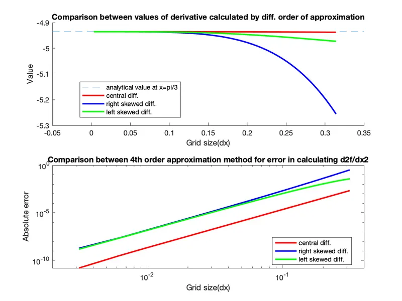
Inference: 1. In the first plot, we can see that the value of all the approximation approaches towards the analytically calculated value as the value of 'dx' decreases.

2. In the second plot, we can see that error via central difference method is the lowest compared to the other two.