Week 8 - Simulation of a backward facing step in OpenFOAM

Objective:

1)To simulate an incomressible laminar viscous flow thoriugh a backward facing step geometry as transient a transient case .

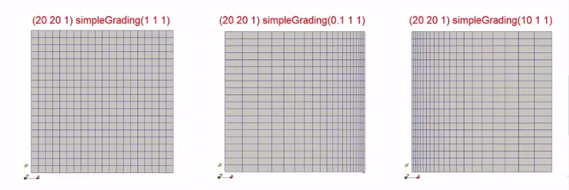
2) Case 1 - Simulate the flow without using any grading factor (i.e., GF = 1)

3)Case 2 - Simulate the flow with grading factor of 0.2. The cells should be finer near the walls (includig the step wall).

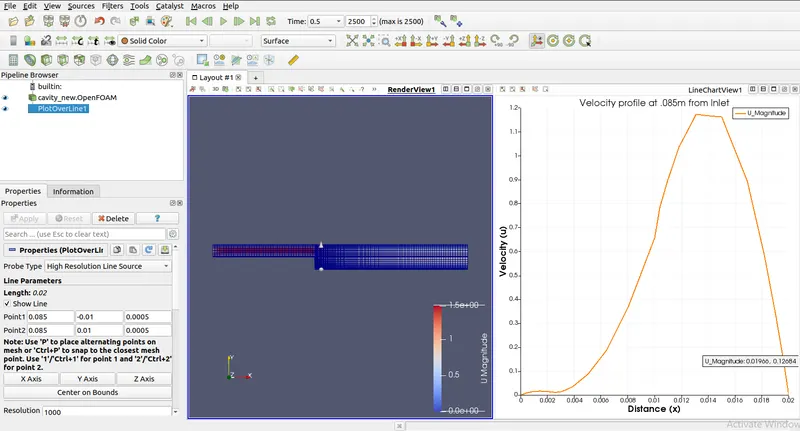
4) To measure velocity profile at 0.85m from inlet for both cases and compare .

5) Explain imortance of grading factor .

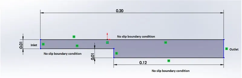
Given geometry

Theory :

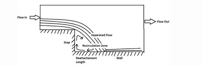
The given case is an incomressibel laminar viscous flow .

The implication of each term is mentioned below :

a) Incomressible : It means that the density of the fluid remains constant for isothermal pressure changes i.e for which the co-efficient of compressibility is 0 .

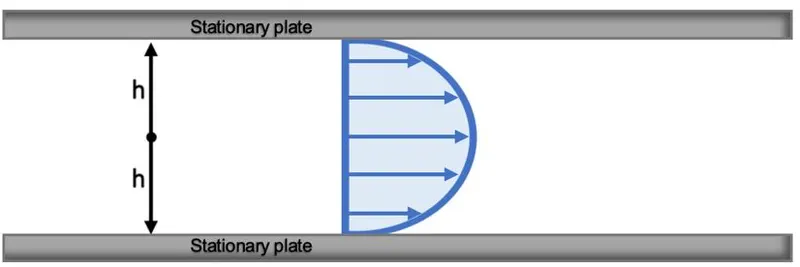
b) Laminar : This implies that the fluid flow is in streamline or the fluid properties like velocity , pressure etc remains constant at any point along the flow . The fluid in contact with horizontal surface is stationary , while all other layers slide over each other .Laminar flow in a straight pipe may be considered as the relative motion of a set of concentric cylinders of fluid, the outside one fixed at the pipe wall and the others moving at increasing speeds as the centre of the pipe is approached. Velocity profile of the fluid in a laminar flow is given below .

c) Viscous : This term implies that the fluid has a high viscosity i.e it does not flow easily .

Governing Equations :

Since it is an incompressible fluid ,

Continuity equation `nabla.u=0`

The momentum equation is divided by density `rho` on both sides , hence we get

Momentum equation `(delu)/(delt) + nabla.(u.u) = -1/(rho).nabla.barp + nabla.nu [2S]`

`(delu)/(delt)` represents the transient nature of the flow .

Since the flow is laminar, there is no turbulence term in the momentum equation .

`nu` is the kinematic viscosity .

Case set up :

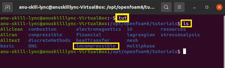
step1 : Access the necessary files from tutorial folder . File path which meets the required condition tutorial>incomressible>icoFoam>cavity .

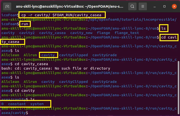
step2 : Copy the necessry folder into a new folder (RUN ) .

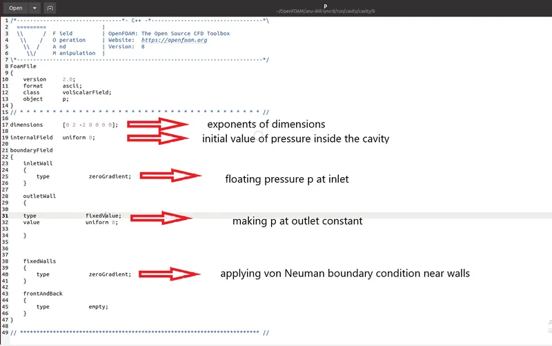
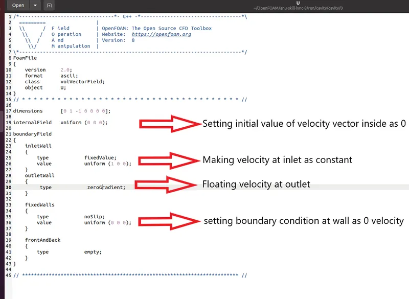
Step 2 : set up initial conditons inside the folder 0 .

At inlet we float pressure and keep velocity constant and at outlet , we float velocity , keeping the pressure constant.

Step 3 : Mesh set up .

The mesh is set up according to the given conditions . We edit the following parameters inside system folder .

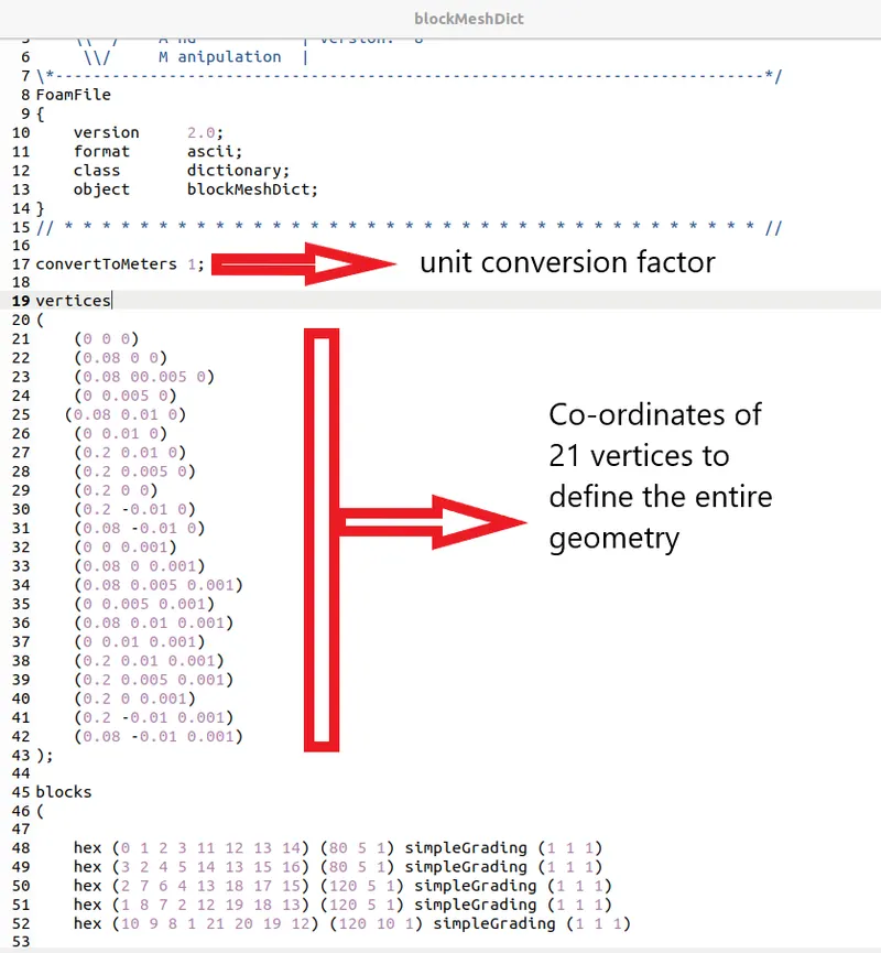
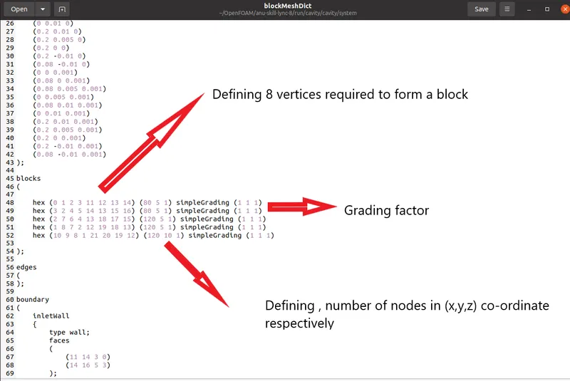
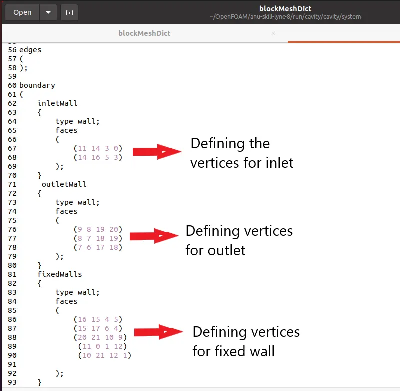
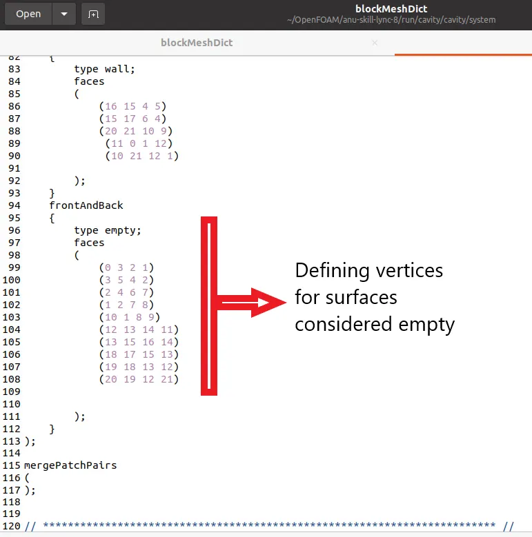
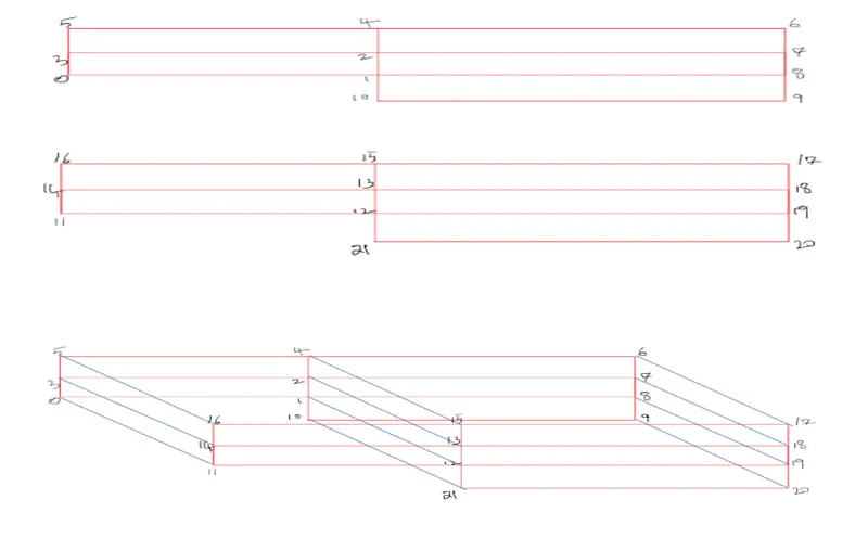
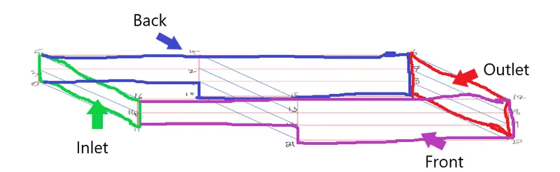
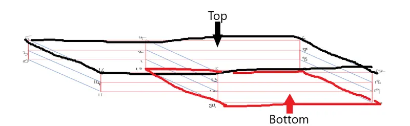
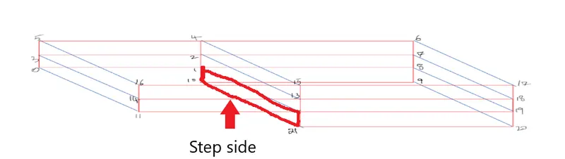
Hence we have rendered the geometery as per give conditions .

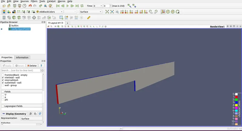
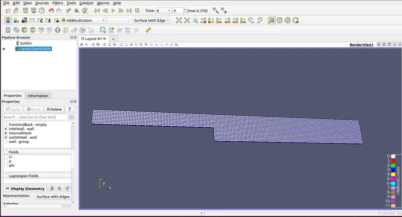
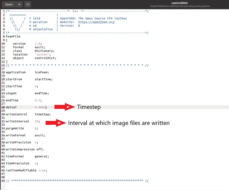
step 4 : Setting up timestep .

In order to set up time step , we open the controlDict file in system .

step 5 : Now we run the solver using icoFoam command inside the run folder . This solves the simulation using entered parameters .

and we can view the results using paraFoam command .

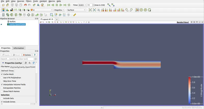
Output :

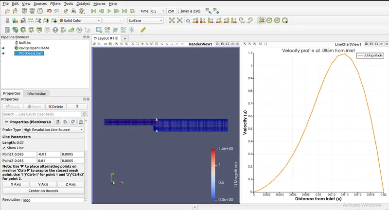
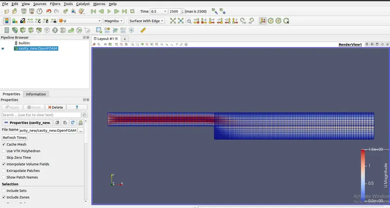
case 1 : Without using any grading factor

case2 :

In case 2 , we gave applied a grading factor of 0.2 along all the walls .

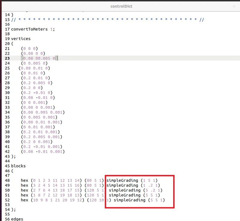
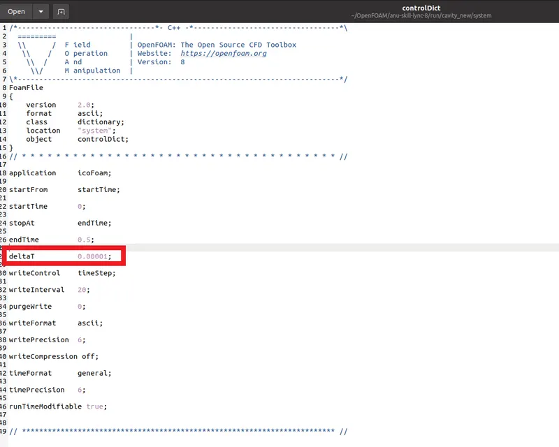
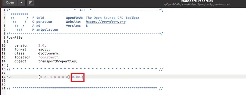
Since we have changed the grading factor , we need to change time step , as well as kinematic viscosity to meet CFL number criteria .

We have reduced the time step to .00001 from .001

and have changed the `nu` value to .001 from .01 .

Inference :

a) We can oberve that the velocity is highest at the center area ,equidistant from both the walls till it reaches the step .

Once the flow reaches the step , the velocity reduces as the area increases .

b)We can observe that the velocity profile is very similar for both the cases .

The case with simple grading factor of (1 1 1) produces a much smoother curve . Whereas the second case produces slight edges at some areas beacuse of the coarse mesh in those regions .

The grading factor does not produce any significant result in this particular case .

Grading factor = length of last cell / length of first cell