Week 8 - Simulation of a backward facing step in OpenFOAM
In this challenge, you are going to simulate an incompressible-laminar-viscous flow through the backward facing step geometry. You should perform a transient simulation. The solver can be chosen based on the described physics of the flow. You need to explain the entire simulation procedure (how you set up the case). You should also provide explanations to every change you make inside the reference case files obtained from OpenFOAM tutorials. You can choose the inlet velocity shuch that the flow is laminar.
After that, you will perform 2 case studies as described below and compare the results.
Case 1 - Simulate the flow without using any grading factor (i.e., GF = 1)
Case 2 - Simulate the flow with grading factor of 0.2. The cells should be finer near the walls (includig the step wall).
You can use the following mesh parameters but you can feel free to modify these values.
Mesh specification
- Number of cells along the x direction (longer dimension) = 200
- Number of cells along the longer y direction = 20;
Boundary condition specification
The domain specifications are provided in the following figure.
Start the terminal in the Linux operating system by using the ctrl+alt+T keyboard shortcut or by selecting Open Terminal from the context menu. You will get the following window after running the terminal.
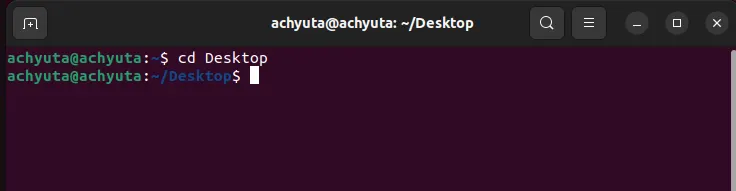
Simply enter "tut" to access the OpenFOAM tutorial directory. At this point, we need to simulate our issue in openFOAM and solve it using one of the program's tutorials. To see what sort of tutorials are included in this directory, enter "ls."
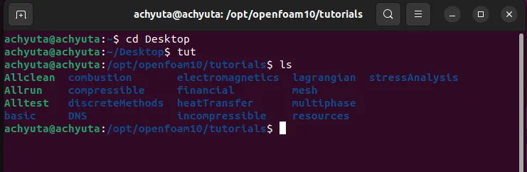
In order to tackle this issue, we must perform an incompressible flow simulation. To do this, type "cd incompressible" to open the incompressible directory, and then "ls" to see the folder structure inside that directory.
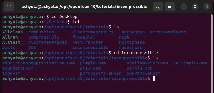
We can observe the abundance of solver folders in the image above. We need a laminar-viscous flow solver for this specific problem. Thus, we choose "icoFoam" here.
The openFoam solver icoFoam is used as a transient solution for Newtonian fluids with incompressible, laminar flow.
As a result, we will choose the icoFoam folder by entering "cd icoFoam," and we will then examine this folder in the terminal by typing "ls."
In cavity, we are, again, going to see cavity folder, where we have to define our fluid domain and generate block mesh.
But we are not going to make any changes here in tutorial section. First of all, OpenFoam does no let anyone make any changes in their official tutorial and secondly, any changes with their official tutorials my corrupt openFoam. An in a bid to correct it, we may need to reinstall open foam all over again.
So, we are going to copy this cavity folder using ‘cp -r cavity’ command and paste it in openFoam run folder by typing ‘cp -r cavity $FOAM_RUN/cavity1’.
And then open run folder by typing ‘cd $FOAM_RUN’. where we can see cavity_test file.
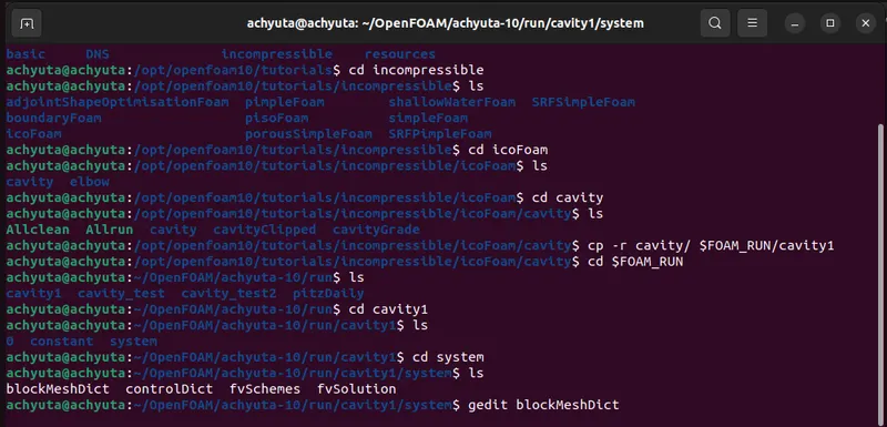
Changes to the cavity1 file may now be made without ever impacting the openFoam official files. Click the cavity test folder. Here, we may specify where to put our block mesh's specifications in the system folder. We can build a domain and provide the necessary block mesh specifications. Therefore, use "gedit blockMeshDict" to open this file and make the c++ program as per our requirements.
/*--------------------------------*- C++ -*----------------------------------*\

  =========                 |

  \\      /  F ield         | OpenFOAM: The Open Source CFD Toolbox

   \\    /   O peration     | Website:  https://openfoam.org

    \\  /    A nd           | Version:  10

     \\/     M anipulation  |

\*---------------------------------------------------------------------------*/

FoamFile

{

    format      ascii;

    class       dictionary;

    object      blockMeshDict;

}

// * * * * * * * * * * * * * * * * * * * * * * * * * * * * * * * * * * * * * //


convertToMeters 0.01;


vertices

(

    (0 0 0)   //0

    (8 0 0)   //1

    (8 0.5 0) //2

    (0 0.5 0) //3

    (8 1 0)   //4

    (0 1 0)   //5

    (20 1 0)  //6

    (20 0.5 0)//7

    (20 0 0)  //8

    (20 -1 0) //9

    (8 -1 0)  //10

    (0 0 0.1) //11

    (8 0 0.1)  //12

    (8 0.5 0.1)//13

    (0 0.5 0.1)//14

    (8 1 0.1)  //15

    (0 1 0.1)  //16

    (20 1 0.1) //17

    (20 0.5 0.1)//18

    (20 0 0.1)  //19

    (20 -1 0.1) //20

    (8 -1 0.1)  //21

);


blocks

(

    hex (0 1 2 3 11 12 13 14) (200 20 1) simpleGrading (1 1 1)  //block1

    hex (3 2 4 5 14 13 15 16) (200 20 1) simpleGrading (1 1 1)  //block2

    hex (2 7 6 4 13 18 17 15) (200 20 1) simpleGrading (1 1 1)  //block3

    hex (1 8 7 2 12 19 18 13) (200 20 1) simpleGrading (1 1 1)  //block4

    hex (10 9 8 1 21 20 19 12) (200 20 1) simpleGrading (1 1 1)  //block5

);


boundary

(

    inlet

    {

        type wall;

        faces

        (

            (0 11 14 3)

            (3 14 16 5)

        );

    }

    outlet

    {

        type wall;

        faces

        (

            (9 8 19 20)

            (8 7 18 19)

            (7 6 17 18)

        );

    }


    frontAndBack

    {

    	type empty;

    	faces

    	(

    		(11 12 13 14)

    		(14 13 15 16)

    		(13 18 17 15)

    		(12 19 18 13)

    		(21 20 19 12)

    		(0 3 2 1)

    		(3 5 4 2)

    		(2 4 6 7)

    		(1 2 7 8)

    		(10 1 8 9)

    	);

    }

    fixedWalls

    {

        type wall;

        faces

        (

            (5 16 15 4)

            (0 1 12 11)

            (4 15 17 6)

            (10 9 20 21)

            (10 21 12 1)

        );

    }

);


mergePatchPairs

(

);


// ************************************************************************* //
Vertices:-
After that, we offer a list of vertices in codes by specifying their x, y, and z coordinates; it always starts with a vertex (0,0,0). Therefore, we must design the following geometry. Let's think about building the geometry shown in the above picture using 5 blocks, as shown in the figure below.

Now, we are going to provide vertices for each block by referring the following sketch.
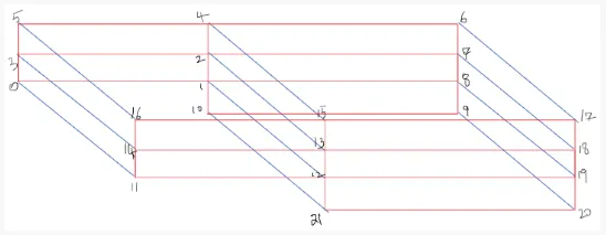
vertices
(
    (0 0 0)       //0
    (8 0 0)       //1
    (8 0.5 0)     //2
    (0 0.5 0)     //3
    (8 1 0)       //4
    (0 1 0)       //5
    (20 1 0)      //6
    (20 0.5 0)    //7
    (20 0 0)      //8
    (20 -1 0)     //9
    (8 -1 0)      //10
    (0 0 0.1)     //11
    (8 0 0.1)     //12
    (8 0.5 0.1)   //13
    (0 0.5 0.1)   //14
    (8 1 0.1)     //15
    (0 1 0.1)     //16
    (20 1 0.1)    //17
    (20 0.5 0.1)  //18
    (20 0 0.1)    //19
    (20 -1 0.1)   //20
    (8 -1 0.1)    //21
);
We will define a block for meshing next. The word "hex," which appears in block parenthesis as the first letter of the mesh format, designates the hexahedral mesh as the kind of mesh. Then, once again in parenthesis, we provide the number of vertices in the order that adheres to the right-hand thumb rule. In other words, the thumb serves as the z-axis, and the order of the vertices is determined by the rotational order of our other finger. The amount of mesh grids that we wish to split into x, y, and z lengths follows. It is defined as the (nx, ny, nz) format.
Grading factor or expansion ratios:-
The expansion ratios enable the mesh to be graded, or refined, in specified directions. The ratio is that of the width of the end cell
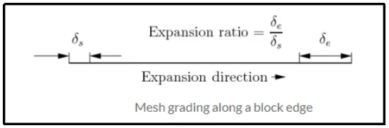
Next, establish the problem's perimeter. Here, we must specify the 3D block's faces, which must be arranged in accordance with the right-hand rule. Set the following faces for this issue.
blocks
(
    hex (0 1 2 3 11 12 13 14) (200 20 1) simpleGrading (1 1 1)   // block1
    hex (3 2 4 5 14 13 15 16) (200 20 1) simpleGrading (1 1 1)   // block2
    hex (2 7 6 4 13 18 17 15) (200 20 1) simpleGrading (1 1 1)   // block3
    hex (1 8 7 2 12 19 18 13) (200 20 1) simpleGrading (1 1 1)   // block4
    hex (10 9 8 1 21 20 19 12) (200 20 1) simpleGrading (1 1 1)  // block5
);
edges
(
);
boundary
(
inlet
{
type wall;
faces
(
(0 11 14 3)
(3 14 16 5)
);
}
outlet
{
type wall;
faces
(
(9 8 19 20)
(8 7 18 19)
(7 6 17 18)
);
}
frontAndBack
{
type empty;
faces
(
(11 12 13 14)
(14 13 15 16)
(13 18 17 15)
(12 19 18 13)
(21 20 19 12)
(0 3 2 1)
(3 5 4 2)
(2 4 6 7)
(1 2 7 8)
(10 1 8 9)
);
}
fixedWalls
{
type wall;
faces
(
(5 16 15 4)
(0 1 12 11)
(4 15 17 6)
(10 9 20 21)
(10 21 12 1)
);
}
);
mergePatchPairs
(
);
After modifying, save and exit the blockMeshDic file.
Additionally, we will modify the "controlDict" file to include start and finish times for time limitations. also to symbolise deltat. Although choosing a deltat CFL value that is smaller than 1 is preferred. Otherwise, the solution could abruptly come to an end or it might diverge just as it is about to converge. Therefore, modify the "controlDict" file as follows.
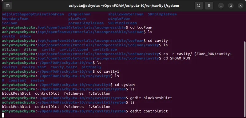
Edit codes following way
/*--------------------------------*- C++ -*----------------------------------*\

  =========                 |

  \\      /  F ield         | OpenFOAM: The Open Source CFD Toolbox

   \\    /   O peration     | Website:  https://openfoam.org

    \\  /    A nd           | Version:  10

     \\/     M anipulation  |

\*---------------------------------------------------------------------------*/

FoamFile

{

    format      ascii;

    class       dictionary;

    location    "system";

    object      controlDict;

}

// * * * * * * * * * * * * * * * * * * * * * * * * * * * * * * * * * * * * * //


application     icoFoam;


startFrom       startTime;


startTime       0;


stopAt          endTime;


endTime         0.2;


deltaT          0.00001;


writeControl    timeStep;


writeInterval   20;


purgeWrite      0;


writeFormat     ascii;


writePrecision  6;


writeCompression off;


timeFormat      general;


timePrecision   6;


runTimeModifiable true;


// ************************************************************************* //
The next step is to establish the starting values for velocity and pressure. In order to achieve so, we must use the 'cd..' command to return to the cavity1 directory and choose the starting values folder, which is designated "0". Initial pressure and velocity values in this situation.
Initial setting for Velocity
/*--------------------------------*- C++ -*----------------------------------*\

  =========                 |

  \\      /  F ield         | OpenFOAM: The Open Source CFD Toolbox

   \\    /   O peration     | Website:  https://openfoam.org

    \\  /    A nd           | Version:  10

     \\/     M anipulation  |

\*---------------------------------------------------------------------------*/

FoamFile

{

    format      ascii;

    class       volVectorField;

    object      U;

}

// * * * * * * * * * * * * * * * * * * * * * * * * * * * * * * * * * * * * * //


dimensions      [0 1 -1 0 0 0 0];


internalField   uniform (0 0 0);


boundaryField

{

    inlet

    {

        type            fixedValue;

        value           uniform (1 0 0);

    }


    outlet

    {

        type            zeroGradient;

    }


   fixedWalls

   {

   	type		noSlip;

   	value		uniform (0 0 0);

   }

     frontAndBack

    {

        type            empty;

    }

}


// ************************************************************************* //
Initial setting for Pressure
/*--------------------------------*- C++ -*----------------------------------*\

  =========                 |

  \\      /  F ield         | OpenFOAM: The Open Source CFD Toolbox

   \\    /   O peration     | Website:  https://openfoam.org

    \\  /    A nd           | Version:  10

     \\/     M anipulation  |

\*---------------------------------------------------------------------------*/

FoamFile

{

    format      ascii;

    class       volScalarField;

    object      p;

}

// * * * * * * * * * * * * * * * * * * * * * * * * * * * * * * * * * * * * * //


dimensions      [0 2 -2 0 0 0 0];


internalField   uniform 0;


boundaryField

{

    inlet

    {

        type            zeroGradient;

    }


    outlet

    {

        type            fixedValue;

        value            uniform 0;

    }


    fixedWalls

    {

    	type		zeroGradient;

    }


    frontAndBack

    {

        type            empty;

    }

}


// ************************************************************************* //
Now that the issue statement has been established, we can deploy the mesh using the 'blockMesh' command and then use the 'checkMesh' function to see whether our mesh has any errors.
blockMesh
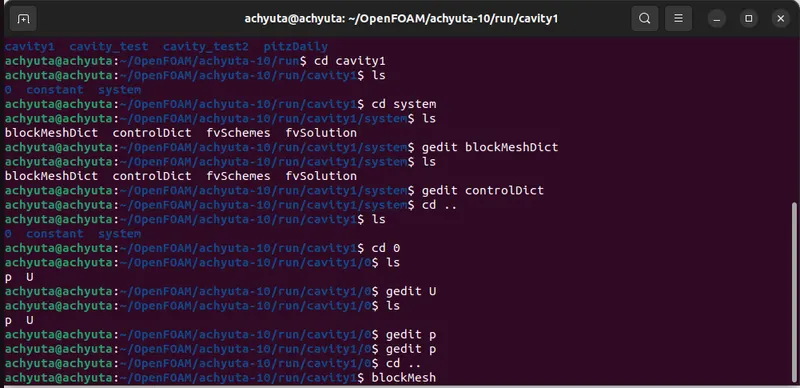
checkMesh
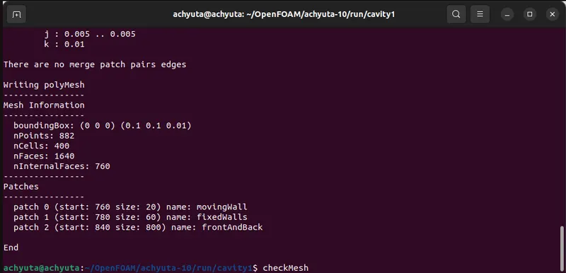
Now that the mesh has been deployed, we are prepared to begin the simulation. We decided on the simulation icoFoam. So, just enter "icoFoam" to begin the simulation.
let us view the results in paraView by using ‘paraFoam’ command
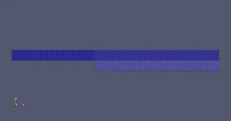
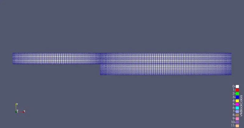
Mesh distribution
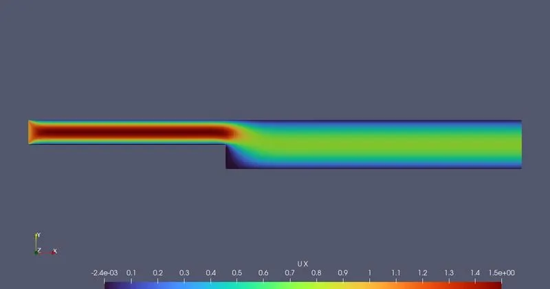
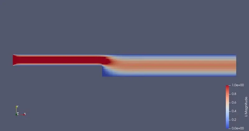
Velocity Distribution along the x axis
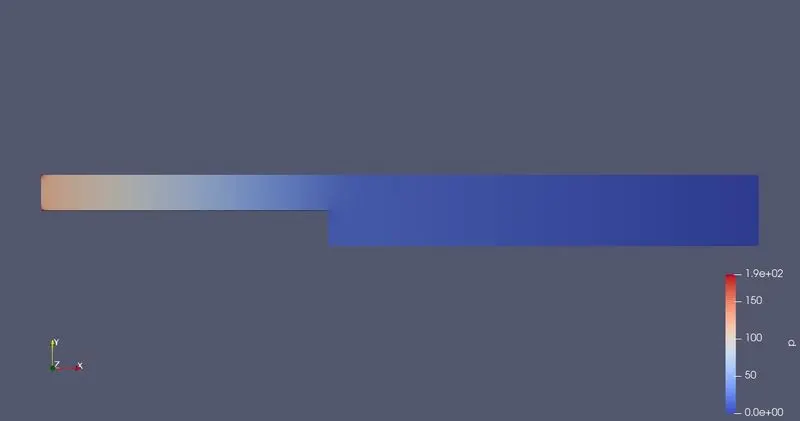
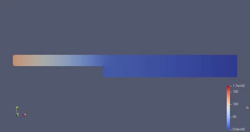
Pressure Distribution along the x axis
Calculate velocity at distance 0.085m from the inlet and plot the graph
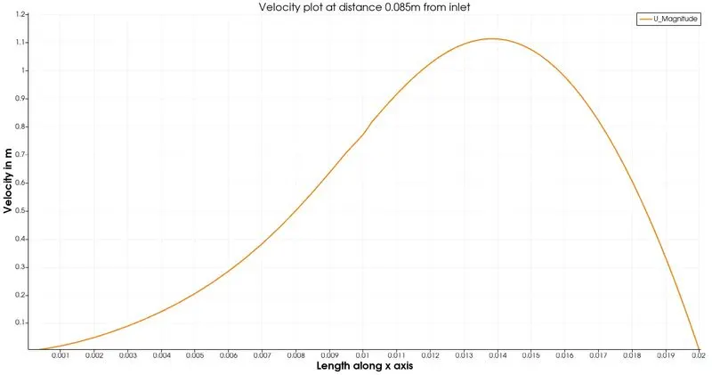
With Grading Factor 0.2 (cell near All walls)
/*--------------------------------*- C++ -*----------------------------------*\

  =========                 |

  \\      /  F ield         | OpenFOAM: The Open Source CFD Toolbox

   \\    /   O peration     | Website:  https://openfoam.org

    \\  /    A nd           | Version:  10

     \\/     M anipulation  |

\*---------------------------------------------------------------------------*/

FoamFile

{

    format      ascii;

    class       dictionary;

    object      blockMeshDict;

}

// * * * * * * * * * * * * * * * * * * * * * * * * * * * * * * * * * * * * * //


convertToMeters 0.01;


vertices

(

    (0 0 0)   //0

    (8 0 0)   //1

    (8 0.5 0) //2

    (0 0.5 0) //3

    (8 1 0)   //4

    (0 1 0)   //5

    (20 1 0)  //6

    (20 0.5 0)//7

    (20 0 0)  //8

    (20 -1 0) //9

    (8 -1 0)  //10

    (0 0 0.1) //11

    (8 0 0.1)  //12

    (8 0.5 0.1)//13

    (0 0.5 0.1)//14

    (8 1 0.1)  //15

    (0 1 0.1)  //16

    (20 1 0.1) //17

    (20 0.5 0.1)//18

    (20 0 0.1)  //19

    (20 -1 0.1) //20

    (8 -1 0.1)  //21

);


blocks

(

    hex (0 1 2 3 11 12 13 14) (80 5 1)                               // block1

    simpleGrading

    (

        (

            (0.5 0.5 5)

            (0.5 0.5 0.2)

        )

        (

            (0.8 0.9 5)

            (0.2 0.1 1)

        )

        1

    )

    hex (3 2 4 5 14 13 15 16) (80 5 1)                              // block2

    simpleGrading

    (

        (

            (0.5 0.5 5)

            (0.5 0.5 0.2)

        )

        (

            (0.2 0.1 1)

            (0.8 0.9 0.2)

        )

        1

    )

    hex (2 7 6 4 13 18 17 15) (120 5 1)                            // block3

    simpleGrading

    (

        (

            (0.5 0.5 5)

            (0.5 0.5 0.2)

        )

        (

            (0.2 0.1 1)

            (0.8 0.9 0.2)

        )

        1

    )

    hex (1 8 7 2 12 19 18 13) (120 5 1)                            // block4

    simpleGrading

    (

        (

            (0.5 0.5 5)

            (0.5 0.5 0.2)

        )

        (

            (0.8 0.9 5)

            (0.2 0.1 1)

        )

        1

    )

    hex (10 9 8 1 21 20 19 12) (120 10 1)                          // block5

    simpleGrading

    (

        (

            (0.5 0.5 5)

            (0.5 0.5 0.2)

        )

        (

            (0.9 0.9 5)

            (0.1 0.1 1)

        )

        1

    )

);


boundary

(

    inlet

    {

        type wall;

        faces

        (

            (0 11 14 3)

            (3 14 16 5)

        );

    }

    outlet

    {

        type wall;

        faces

        (

            (9 8 19 20)

            (8 7 18 19)

            (7 6 17 18)

        );

    }


    frontAndBack

    {

    	type empty;

    	faces

    	(

    		(11 12 13 14)

    		(14 13 15 16)

    		(13 18 17 15)

    		(12 19 18 13)

    		(21 20 19 12)

    		(0 3 2 1)

    		(3 5 4 2)

    		(2 4 6 7)

    		(1 2 7 8)

    		(10 1 8 9)

    	);

    }

    fixedWalls

    {

        type wall;

        faces

        (

            (5 16 15 4)

            (0 1 12 11)

            (4 15 17 6)

            (10 9 20 21)

            (10 21 12 1)

        );

    }

);


mergePatchPairs

(

);


// ************************************************************************* //
Output mesh from above codes
Velocity Distribution along the x axis
Pressure Distribution along the x axis
Calculate velocity at distance 0.085m from the inlet and plot the graph
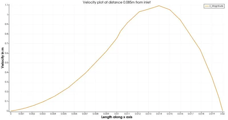
Results
Up till now, we have completed producing velocity charts for both instances with and without a 0.2 grading factor. In comparison to the other two charts, the velocity without grading factor plot seems to be smoother and more accurate when we look at all three line graphs. So, one might claim that grading may affect our outcomes. However, it is untrue. Because, if we look closely, we can see that the mesh is incredibly fine along the X-axis at the step wall yet quite coarse along the Y-axis. As a result, the smooth plot for the velocity at the 0.085 positions on the Y-axis is not there.
After understanding how mesh functions in reality, we need to apply fine mesh close to the area where we anticipate our outcomes. To successfully capture these significant shifts, we must constantly employ grading or a finer mesh close to walls in CFD since fluid always exhibits them there. One should be aware of when to employ finer grading factors in order to acquire effective and trustworthy results. Assume that in an effort to provide more effective outcomes, using a high number of fine components will increase computing time and computational memory requirements (RAM). Grading is crucial since it enables us to employ tiny mesh to capture flow at boundary walls and obstructions and coarse mesh in more open areas. The significance of tiny mesh is also clear from the image below. The resolution of the picture is becoming better as the grading factor rises step by step. This indicates that the flow result increases as the number of elements increases.