Week 8 - Simulation of a backward facing step in OpenFOAM
- Simulate an incompressible-laminar-viscous flow through the backward facing step geometry. You should perform a transient simulation. The solver can be chosen based on the described physics of the flow.
perform 2 case studies as described below and compare the results.
Case 1 - Simulate the flow without using any grading factor (i.e., GF = 1)
Case 2 - Simulate the flow with grading factor of 0.2. The cells should be finer near the walls.
- Objective- To simulate an incompressible-laminar-viscous flow through the backward facing step geometry and also perform the transient simulation.To perform 2 case studies as described below and compare the results.
Case 1 - Simulate the flow without using any grading factor (i.e., GF = 1)
Case 2 - Simulate the flow with grading factor of 0.2. The cells should be finer near the walls (includig the step wall).
- The flow in which density is constant is known as incompressible flow.
- The smooth and streamlined flows are called as laminar flows.
- When the fluid has more resistance to flow then it is called as viscous flow.
- Transient analysis by definition involves loads that are a function of time
- Grading factor is defined as the ratio of last cell distance to the first cell distance.
- Procedure ,1. Blockmesh
2. Checkmesh
3. Solve (icoFoam)
4. Paraview (visualize)
- Steps- Open the openFoam tutorials and find solutions to solve the incompressible laminar viscous flow problem.
- The next step is to copy the required file in the solver and paste it into the OpenFOAM run folder, leaving the official OpenFoam file intact.
- Find out the block network script file to create the domain space and provide the network specification.
- Find the "controlDict" file and edit the simulation start and end time.
- In the initial folder "0", adjust the initial parameter for velocity and pressure according to the surfaces of the given domain.
- Use the blockMesh command to generate the mesh and checkMesh to verify it.
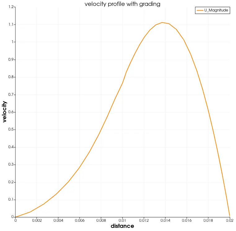
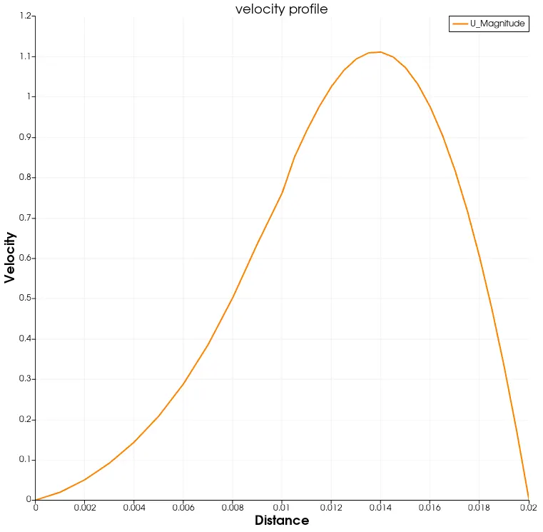
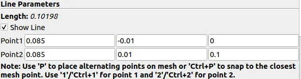
- Open the simulation file in paraView and plot the velocity profile at a point 0.085 m from the inlet.
- Repeat the above procedure for a grading factor of 0.2 to check for differences in results.
Write a detailed report explaining all the commands and codes used in the project. -
Boundary condition specification
The domain specifications are provided in the following figure.
-
OpenFoam has 3 basic folders,namely 0, constant , system.
-
The system folder consist of following categories,
1. BlockMeshDict - Used to create a mesh information.
2. ControlDict - Used to control solver time operations.
3. fvSolutions- Used to assign instructions on how to solve discretized linear equations.
4. fvSchemes- Used to assigned discretization schemes.
-
The constant folder consist of following categories,
1. Polymesh- Polymesh contains mesh information generated by the BlockMeshDict
2. TransportProperties- It contains information of transport coefficients.
3. turbulenceProperties- It contains information about turbulence coefficients.
- The 0 folder consist of following categories,
1. P - It contains BC and IC data for pressure at time t=0.
2. U- It contains BC and IC data for velocity at time t=0.
- SimpleGrading- SimpleGrading defines the expansion ratio or mesh stretching in each local direction(x,y,z).
- The boundary condition is specified in the blockmesh dict file.
-

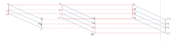
- BlockMeshDict
/*--------------------------------*- C++ -*----------------------------------*\
  =========                 |
  \\      /  F ield         | OpenFOAM: The Open Source CFD Toolbox
   \\    /   O peration     | Website:  https://openfoam.org
    \\  /    A nd           | Version:  10
     \\/     M anipulation  |
\*---------------------------------------------------------------------------*/
FoamFile
{
    format      ascii;
    class       dictionary;
    object      blockMeshDict;
}
// * * * * * * * * * * * * * * * * * * * * * * * * * * * * * * * * * * * * * //

convertToMeters 1;

vertices
(

    (0 0 0)//[0]
    (0.08 0 0)//[1]
    (0.08 0.005 0)//[2]
    (0 0.005 0)//[3]
    (0.08 0.01 0)//[4]
    (0 0.01 0)//[5]
    (0.2 0.01 0)//[6]
    (0.2 0.005 0)//[7]
    (0.2 0 0)//[8]
    (0.2 -0.01 0)//[9]
    (0.08 -0.01 0)//[10]

    (0 0 0.1)//[11]
    (0.08 0 0.1)//[12]
    (0.08 0.005 0.1)//[13]
    (0 0.005 0.1)//[14]
    (0.08 0.01 0.1)//[15]
    (0 0.01 0.1)//[16]
    (0.2 0.01 0.1)//[17]
    (0.2 0.005 0.1)//[18]
    (0.2 0 0.1)//[19]
    (0.2 -0.01 0.1)//[20]
    (0.08 -0.01 0.1)//[21]
);

blocks
(
    hex (0 1 2 3 11 12 13 14) (100 10 1) simpleGrading (0.2 1 1)
    hex (3 2 4 5 14 13 15 16) (100 10 1) simpleGrading (0.2 1 1)
    hex (10 9 8 1 21 20 19 12) (200 10 1) simpleGrading (2 1 1)
    hex (1 8 7 2 12 19 18 13) (200 10 1) simpleGrading (2 1 1)
    hex (2 7 6 4 13 18 17 15) (200 10 1) simpleGrading (2 1 1)
);

edges
(
);

boundary
(
    inlet
   {
        type patch;
        faces
        (
            (0 11 14 3)
            (3 14 16 5)
        );
    }

    outlet
    {
        type patch;
        faces
        (
            (9 8 19 20)
            (8 7 18 19)
            (7 6 17 18)
        );
    }
    Bottomwall
    {
        type wall;
        faces
        (
            (11 0 1 12)
            (21 10 9 20)
            (10 21 12 1)
        );
    }
    Topwall
    {
        type wall;
        faces
        (
           (16 15 4 5)
           (15 17 6 4)
        );
    }


    frontAndBack
    {
        type empty;
        faces
        (
            (14 13 15 16)
            (11 12 13 14)
            (21 20 19 12) //Front side
            (12 19 18 13)
            (13 18 17 15)

            (0 3 2 1)
            (3 5 4 2)
            (2 4 6 7)//Back side
            (1 2 7 8)
            (10 1 8 9)

        );
    }
);
mergePatchPairs
(
);
- ControlDict
- In the controlDict file timesteps can be controlled.
- In this simulation start and end time is provided as 0 and 0.5. deltaT is assumed to be 0.002.
/*--------------------------------*- C++ -*----------------------------------*\
  =========                 |
  \\      /  F ield         | OpenFOAM: The Open Source CFD Toolbox
   \\    /   O peration     | Website:  https://openfoam.org
    \\  /    A nd           | Version:  10
     \\/     M anipulation  |
\*---------------------------------------------------------------------------*/
FoamFile
{
    format      ascii;
    class       dictionary;
    location    "system";
    object      controlDict;
}
// * * * * * * * * * * * * * * * * * * * * * * * * * * * * * * * * * * * * * //

application     icoFoam;

startFrom       startTime;

startTime       0;

stopAt          endTime;

endTime         0.5;

deltaT          0.002;

writeControl    timeStep;

writeInterval   20;

purgeWrite      0;

writeFormat     ascii;

writePrecision  6;

writeCompression off;

timeFormat      general;

timePrecision   6;

runTimeModifiable true;


// ************************************************************************* //- Initial Condition
- The initial condition for velocity and pressure can be provided in the p and U file located in the 0 folder.
- Pressure
/*--------------------------------*- C++ -*----------------------------------*\
  =========                 |
  \\      /  F ield         | OpenFOAM: The Open Source CFD Toolbox
   \\    /   O peration     | Website:  https://openfoam.org
    \\  /    A nd           | Version:  10
     \\/     M anipulation  |
\*---------------------------------------------------------------------------*/
FoamFile
{
    format      ascii;
    class       volScalarField;
    object      p;
}
// * * * * * * * * * * * * * * * * * * * * * * * * * * * * * * * * * * * * * //

dimensions      [0 2 -2 0 0 0 0];

internalField   uniform 0;

boundaryField
{
    inlet
    {
        type            zeroGradient;
    }

    outlet
    {
        type            fixedValue;
        value           uniform 0;
    }

    Bottomwall
    {
        type            zeroGradient;
    }

    Topwall
    {
        type            zeroGradient;
    }

    frontAndBack
    {
        type              empty;
    }

// ************************************************************************* //
Velocity-
/*--------------------------------*- C++ -*----------------------------------*\
  =========                 |
  \\      /  F ield         | OpenFOAM: The Open Source CFD Toolbox
   \\    /   O peration     | Website:  https://openfoam.org
    \\  /    A nd           | Version:  10
     \\/     M anipulation  |
\*---------------------------------------------------------------------------*/
FoamFile
{
    format      ascii;
    class       volVectorField;
    object      U;
}
// * * * * * * * * * * * * * * * * * * * * * * * * * * * * * * * * * * * * * //

dimensions      [0 1 -1 0 0 0 0];

internalField   uniform (0 0 0);

boundaryField
{
    inlet
    {
        type            fixedValue;
        value           uniform (1 0 0);
    }

   outlet
    {

       type             zeroGradient;
    }

    Bottomwall

    {
        type            noSlip;
    }

    Topwall

    {
        type            noSlip;
    }

    frontAndBack
    {
        type            empty;
    }
}

// ************************************************************************* //- Procedure
- Open terminal by clicking clt+alt+T on Linux operating system.
- In a terminal window, type $FOAM_TUTORIALS or TUT.
- ls represents a directory with a list.
- pwd represents the current working directory.
- Type cd incompressible/icoFoam/cavity to enter in cavities folder.
- Copy the cavity directory with cp and paste the directory into RUN
- Enter the RUN window by typing cd $FOAM_RUN.
- In the RUN window, type cd cavity/cavity/system to enter the system folder.
- The notepad.exe command is used to open text files.
- notepad.exe blockmeshdict is used to open a blockmesh file.
- notepad.exe controldict is used to open the controldict file.
- Cd .. is used to go to the previous folder.
- Constants related to fluid flow, such as diffusivity, can be changed in the constants component.
- The initial state related to the fluid flow can be changed under the 0 component.
- Geometry:
The block mesh dict is used to create the geometry, generate the mesh and define the boundary condition. The following procedures should be followed when creating geometry in Blockmesh.
-
The entire piece is created by combining 5 blocks.
-
First, vertices should be defined for each block.
-
After the blocks are created, meshing is done using hex(a,b,c,..) (x,y,z) simpleGrading(p,q,r)
-
Hex represents a hexahedral mesh.
-
a,b,c represent the vertices of the block.
-
x,y,z represents meshing in x,y and z direction.
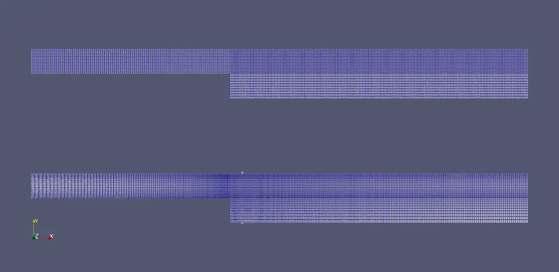
- Results - Mesh with grading and without grading
- Plot -Velocity profile with grading factor 0.2
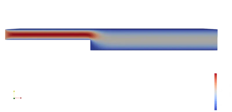
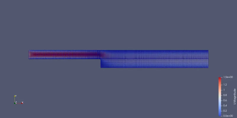
- Velcontour
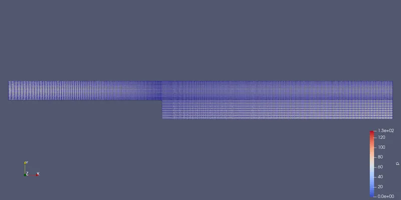
- Precontour

- Plot -Velocity profile with grading factor 1
velcontour
precontour
- To calculate velocity at distance 0.085 from inlet modify following parameters:-
- Results discussion-
- Mesh are generated for grading factor 0.2 and grading factor 1.
- Flow is simulated without using grading factor and with using grading factor 0.2
- Graphs are plotted for the velocity profile.
- When dx value is small ,accuracy increases also as the finer mesh , the more accurate will be the results.
- Explain why Grading/Growth factor is essential for meshing.
- Specifies the maximum ratio of adjacent mesh edges for the transition between coarse and fine regions.
A smaller sorting factor creates a more even mesh.
In the program, we can change the factor in the blockMeshDict code. - SimpleGrading defines the expansion ratio or mesh stretching in each local direction(x,y,z).
- Conclusion:-
- As we can observe from the graphs, there is not much difference between the two meshes.
- But if the values are taken, we can see a slight variation among the two graphs.
- By changing the simple grading factor from 0.2 to 1, the mesh becomes finer and the solution changes to precision.
- Overall, changing the size of the simple grading factor,the result remains the same as approx.
- Execution time is lower for a lower mesh sorting factor.