Week 8 - Simulation of a backward facing step in OpenFOAM

Objective:

Simulate an incompressible—laminar-viscous flow through the Backward facing step geometry. Perform transient simulation; choose solver based on the described flow physics in the problem statement. Explain the simulation process and way of setting up the problem Statement in open Foam and also, explain every change that Has been done inside the reference case files obtained from Open FOAM tutorials. Next, perform two case studies, firstly, form simulation of the flow Without using any grading factor (i.e., CF = 1). Secondly, simulate The flow with a grading factor of 0.2. The cells should be more OK near The walls (including the step wall).

Problem Statement:

Simulate on Incompressible- laminar-viscous flow through the backwards-facing step geometry. Perform 2 case studies as described below and compare the results.

Case 1 - Simulate the flow without using any grading factor (i.e. OF = 1)

Case 2 - Simulate the flow with a grading factor of 0.2. The cells should be lined near the walls (inciudig the step wall).

Mesh specification:

Number of cells along the x direction (longer dimension) = 200

Number of cells along the longer y direction = 20;

Boundary Condition:

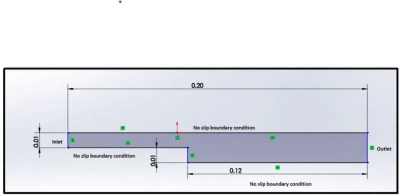
Procedure:

First, we are making the run folder in OpenFOAM where our simulations will be run.

Then we need to copy the cavity folder to the run folder so we can change the blockMeshDict, controlDict, pressure, and velocity files so we can run the simulations we need. We copy the folder because we aren't supposed to change anything in the original folders in OpenFOAM.

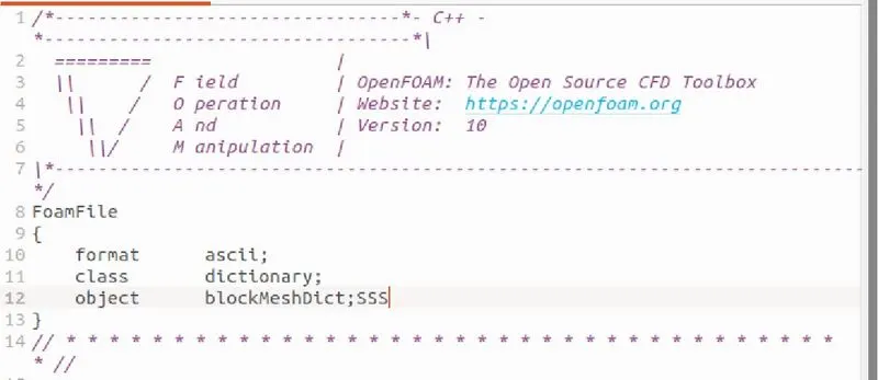
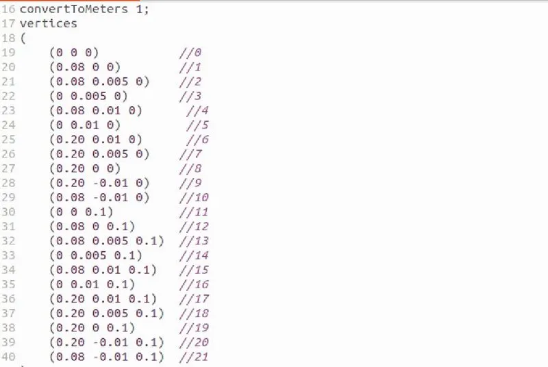
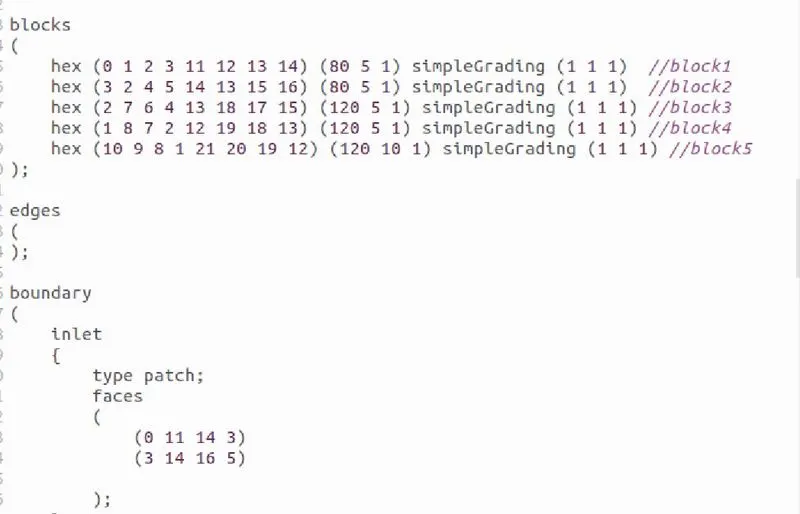
Then, we'll make the necessary changes to the blockMeshDict file, which names the vertices and creates the blocks. In this case, there are 21 vertices and 5 blocks. When creating blocks, we need to say how many mesh points are needed in the x, y, and z directions, and we should also do simple grading along the edges.

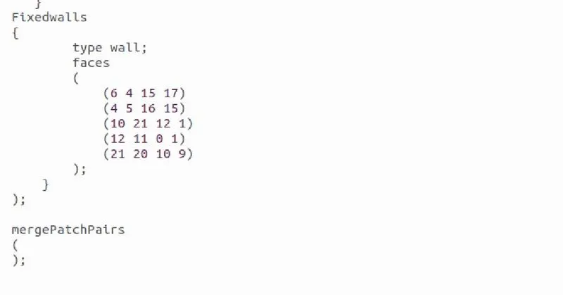
Then, we need to set up the boundary conditions. To do this, we need to define all the faces in OpenFOAM as patches and give them a type. The inlet and outlet will be faces of type patch, the front and back will be faces of type empty, and the top and bottom, which are the boundary conditions in this case, will be faces of type wall. We will save these changes in the blockMeshDict.

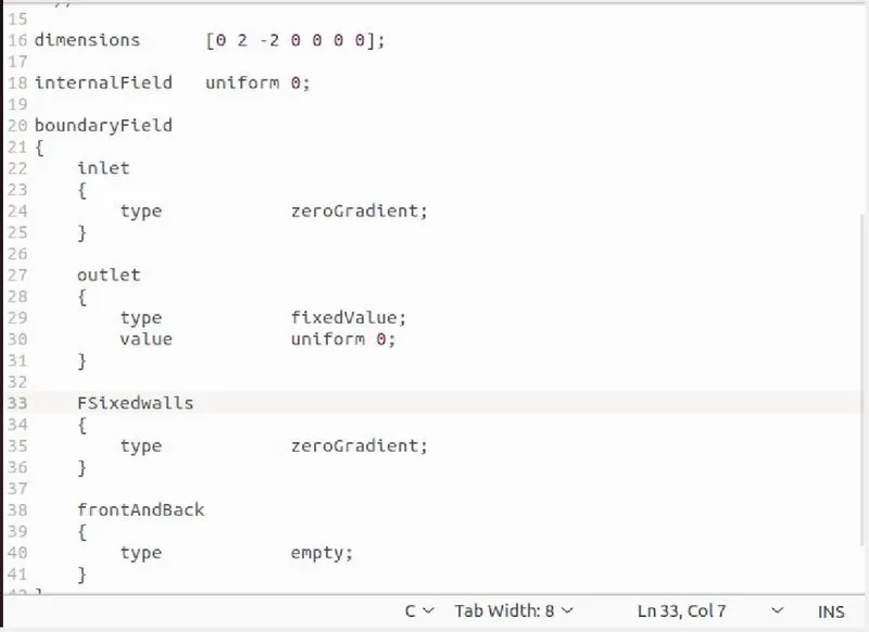
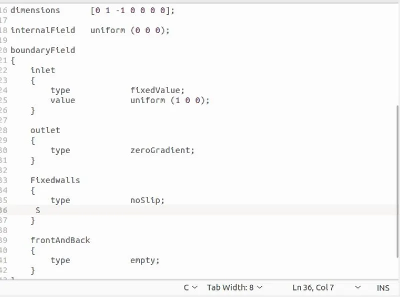
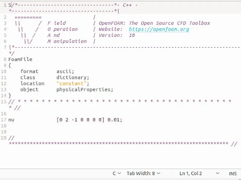
Then, in the velocity and pressure files, we have to say that the velocity at the inlet will be a fixed value, and the pressure will be zerogradient. At the outlet, the velocity will be a fixed value, and the pressure will be a fixed value with a value of 0. The velocity and pressure will be empty at the no-slip boundaries, which are the top and bottom velocity, and at the no-slip boundaries, which are the top and bottom velocity. And we can change the nu value in the transportProperties to get the lower courant number.

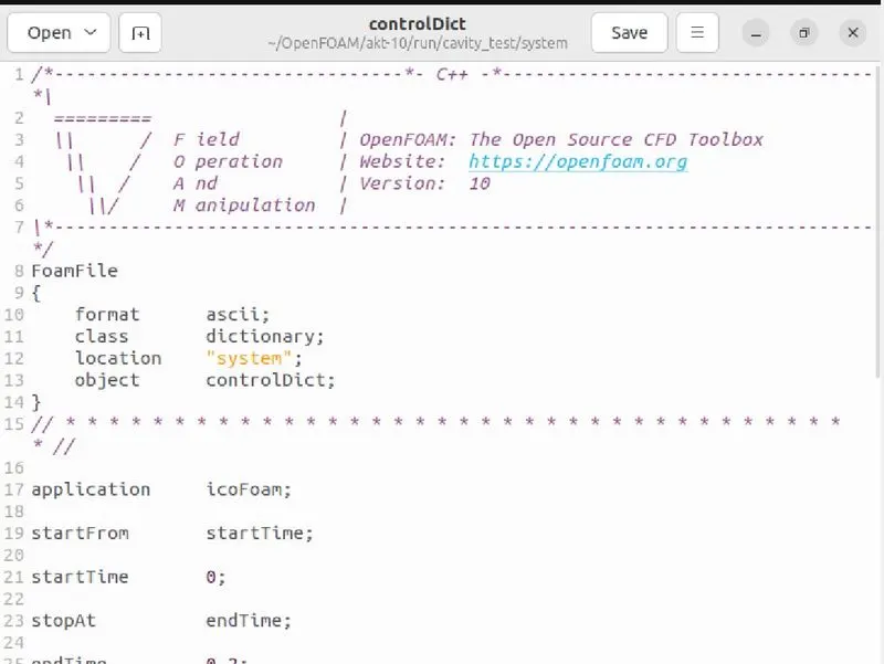
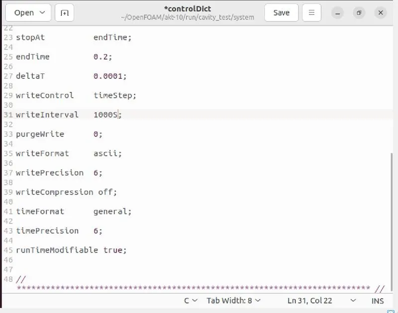
And the simulation time and time step must be set in the controlDict file so that the courant number is less than 0.5.

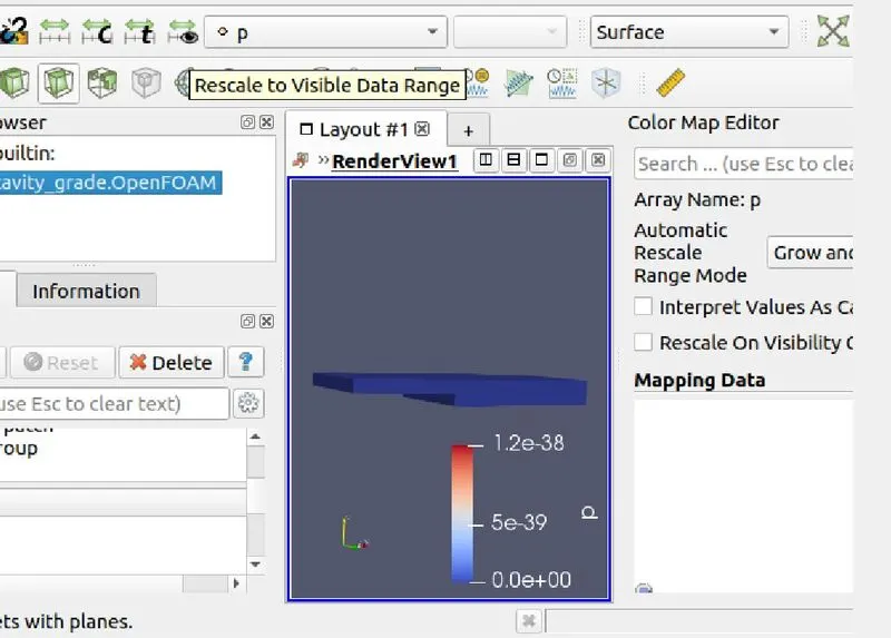
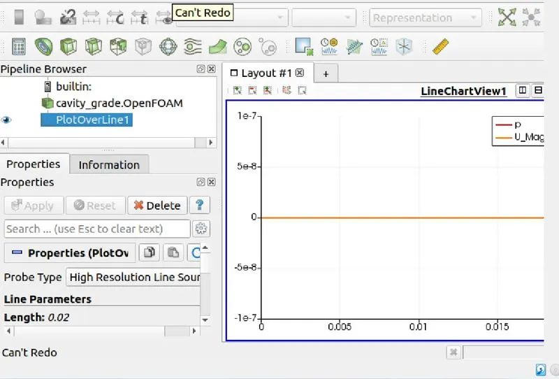
After making the block mesh and running the simulation with the right solver, open the paraview in paraFoam and plot the velocity profile for the given value.

CODES:

Control Dict:

Initial velocity and pressure codes:

Results:

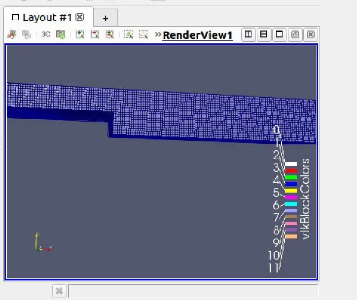
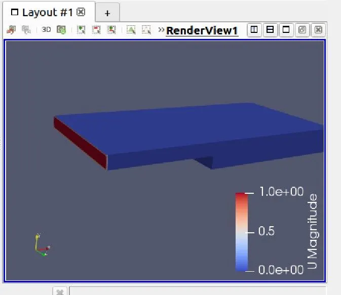
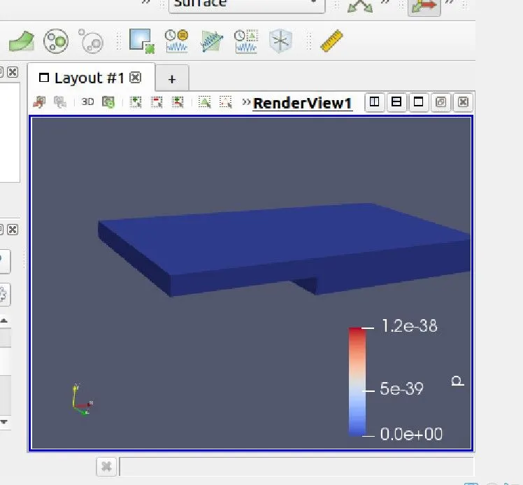
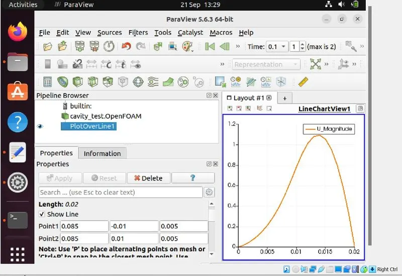
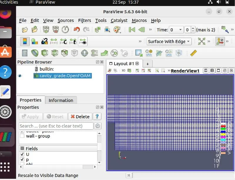
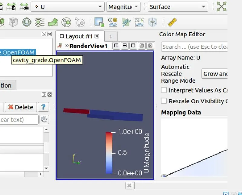
With a Grading factor 0.2:-

Conclusion:

Changing the simple grading factor from 0.2 to 1 makes the mesh finer and the solution more accurate. Overall, the size change of the simple grading factor doesn't change the result. With a lower meshing grading factor, it takes less time to get the material out.