Week 8 - Simulation of a backward facing step in OpenFOAM

Aim:

• set up to simulate an incompressible-laminar-viscous flow through the backward facing step geometry. You should perform a transient simulation.

objective :

• solver can be chosen based on the described physics of the flow.
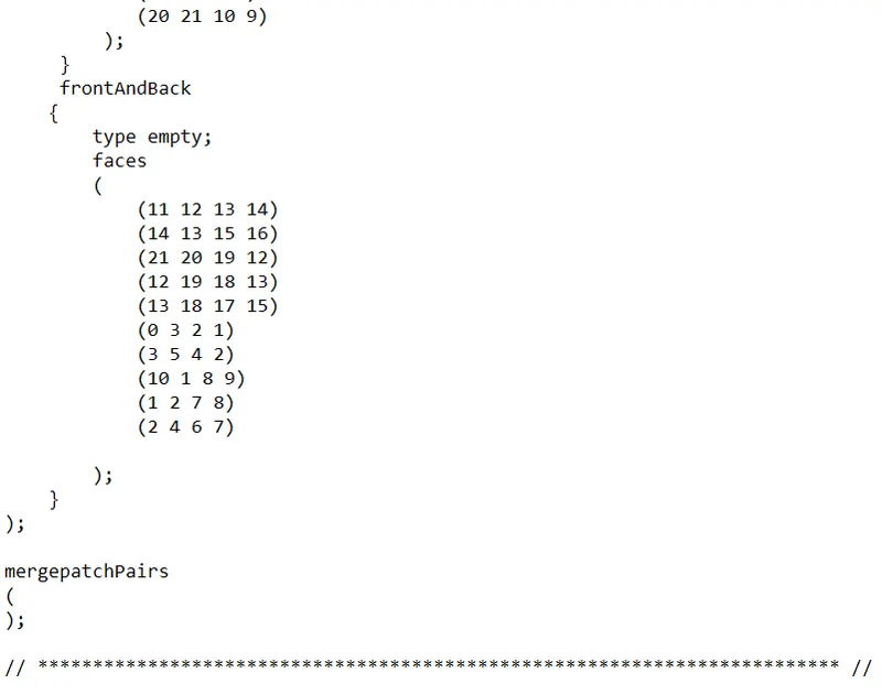
• to explain the entire simulation procedure (how you set up the case).
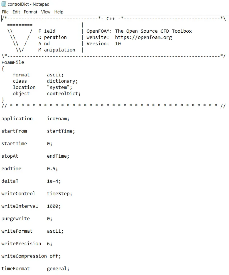
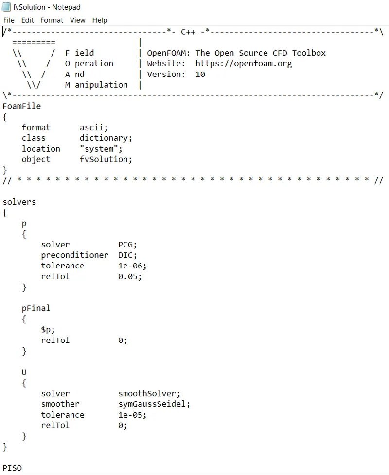
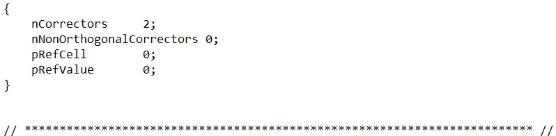
• to provide explanations to every change you make inside the reference case files obtained from OpenFOAM tutorials.
• You can choose the inlet velocity shuch that the flow is laminar.

we will be performing 2 case studies as described below and compare the results.

Case 1 - Simulate the flow without using any grading factor (i.e., GF = 1)

Case 2 - Simulate the flow with grading factor of 0.2. The cells should be finer near the walls (includig the step wall).

We are going to use the following mesh parameters but you can feel free to modify these values.

Mesh specification

1. Number of cells along the x direction (longer dimension) = 200
2. Number of cells along the longer y direction = 20;

Boundary condition specification

The domain specifications are provided in the following figure.

Desired output

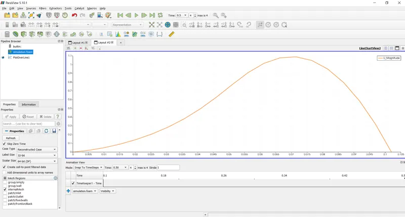
• Measure the velocity profile at 0.085 m from the inlet of the geometry for both case studies and compare. You can use the plot over line tool for this.

to explainwhy Grading/Growth factor is essential for meshing.

Basic definitions :

Theory : Incompressible - laminar - Viscous flow

Incompressible flow : The flow in which there is no change in the density is called the incompressible flow.

Mathematically, an incompressible flow can be expressed as ∇⋅u=0">∇⋅u=0∇⋅u=0

Laminar flow : A laminar flow is one where the fluid motion is regular and there is no mixing . It can be visualized by the pathlines that do not intersect each other.

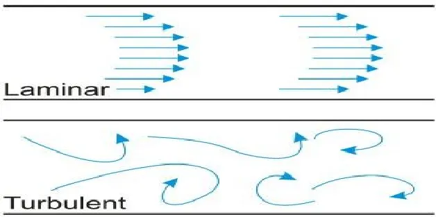
Reynolds number is the parameter to differentiate a flow as laminar or turbulent.

Mathematically, Reynolds number is the ratio of inertial force to the viscous force.

Re=ρ⋅v⋅Lμ">Re=ρ⋅v⋅LμRe=ρ⋅v⋅Lμ

rho corresponds to the density of the fluid.

v is the density of the fluid.

L is the characteristic length of the passage through which the fluid flows. (In case of a fluid flow through the pipe, the charactersitic length is the diameter of the pipe.)

μ">μμis the absolute viscosity of the fluid.

For internal flows of Re ≤">≤≤1000 represent a laminar flow regime`

Viscous flow : Viscosity is the property of fluid by the virtue of which it exhibits a inertia to the fluid motion.

In case of the flow of a viscous fluid a layer of the fluid opposes the motion of another layer of fluid above it. This results in the velocity gradient in the direction perpendicular to the fluid flow.

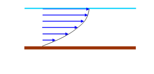
Consider the top layer of fluid moving with the velocity V. However as the fluid is viscous, the layer just underneath it has a velocity less than V. This is because the bottom layer of the fluid exerts an opposition to the movement of the top layer. This results in the velocity gradient across the cross section.

OpenFOAM uses the Finite volume approach to solve the system of the PDE.

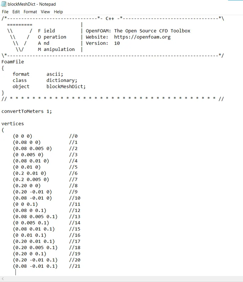
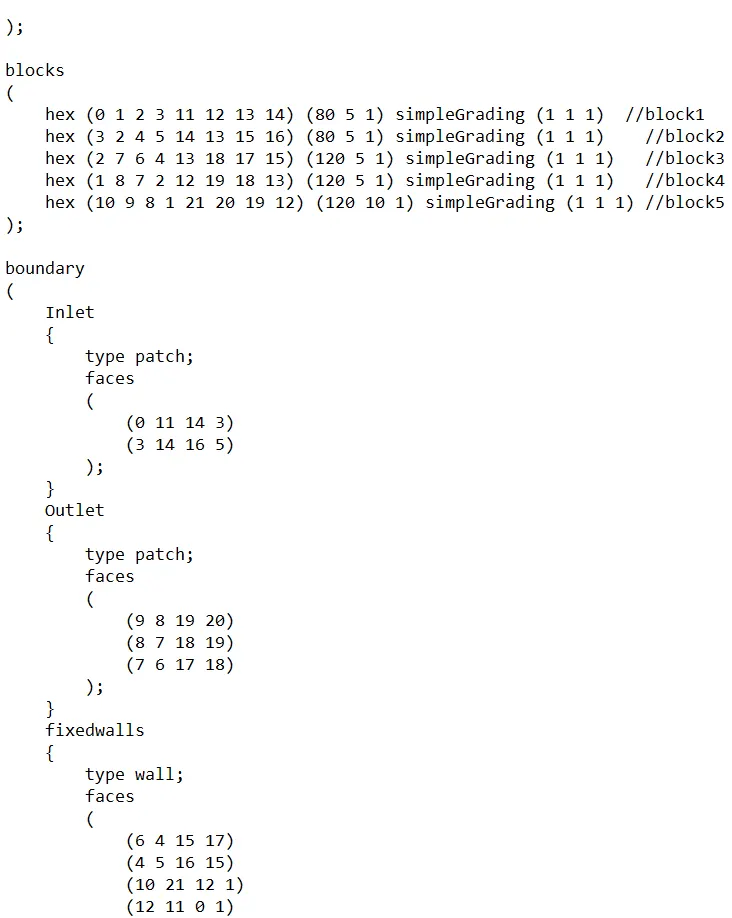
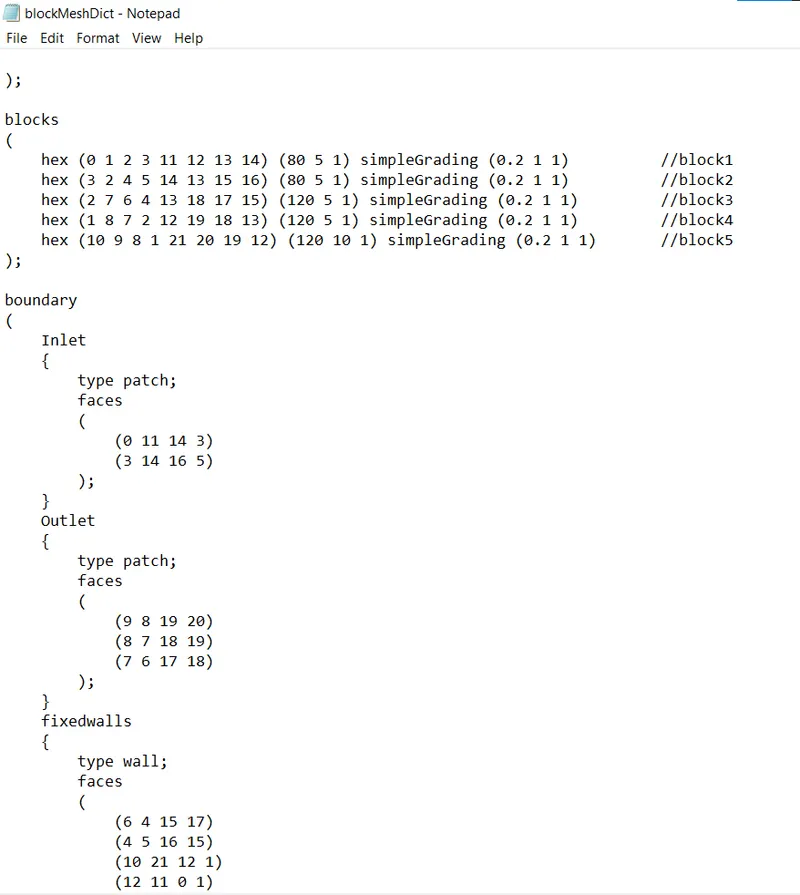
I hve devided this entire block into to 5 small blocks.so the complexity of the problem may increases and we can work with and get more clarity solve similar problems in future.

Theory and explanation of the simulation :

1)we will have to open the ubuntu platform.and start run by using run command

2)later we will have to open the tutorial folder by entering tut command .open this dicectory by using ls command.which will give us liss of the tutorials present inside it.

3)in this directory we will have to select the solver ,here we are choosing icofoam solver ,then we will have to go to the cavity folder which is present inside the icofoam solver then we will have copy that folder by using cp r -cavity %FOAM_RUN command and modify that into as per our block dimensions.

4)then we will have to run the folder.in that we can see that 0,constant,system folders present in side it,we will be having bondary conditions informations of both the pressure and the velocity.and inside the constant folder we will be having an informations of physical properties like viscosity and the turbulance.and finally we will be having blockmeshdict,control dict ,fv schemes ,fv solutions etc.

5)from the given problem we will have to modify the vertices values, the blocks,forward &backward values,inlet and outlet conditions as per the problem statement.

6)after all these things we will have to make sure that in control dict also we will have change the time related variables with respect to the specified time.the time parameters are like intial time and the end time and timeinterval,we will have to make sure that the give time interval satisfies the cfl number or not.we will have to give the better possible values of the time interval by keeping cfl condition in mind.

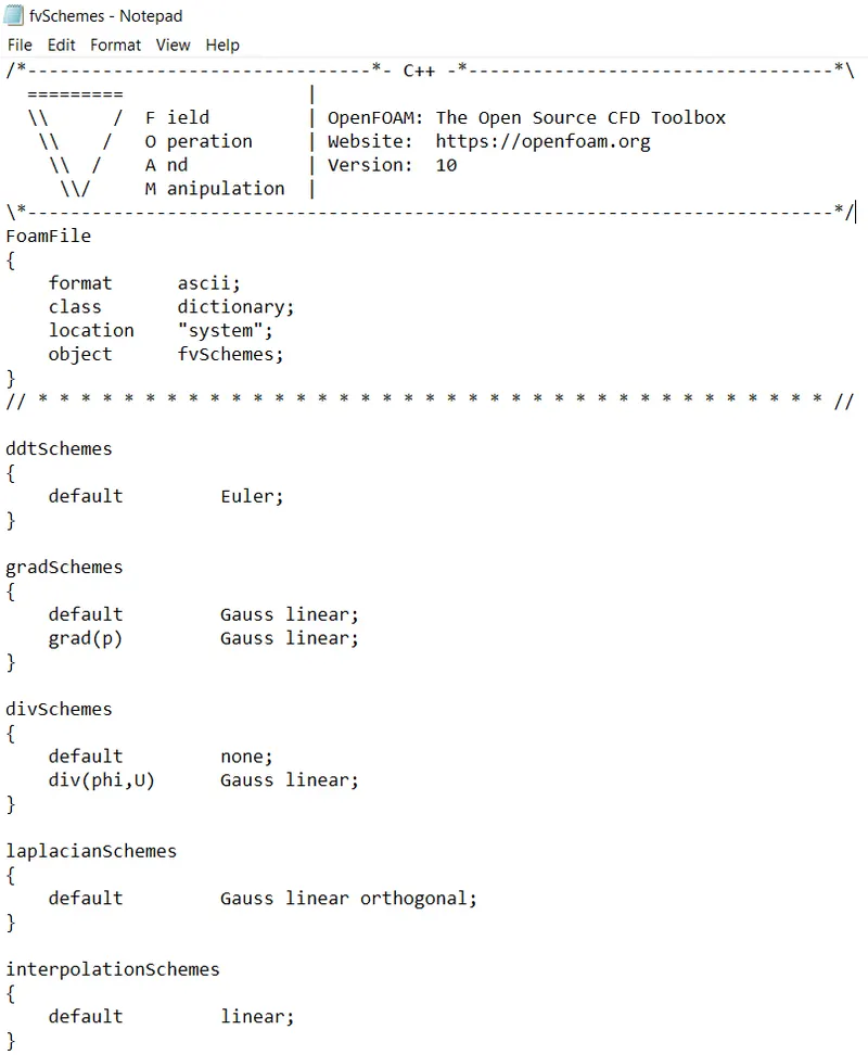
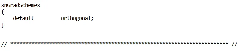
7)The fv schemes ,fv solutions are the folder which gives the information about the what type schemes we have used and what type of solvers we have used.

8)After the the above steps we will have to apply the blockmesh command in ubuntu terminal to ge the meshing details of the specified block.

9)Then we will have to apply the checkmesh to check wheather the mesh is ok or not. if the mesh is good it will gives the confirmation that Mesh is ok.if its not it gives like mesh is not ok.if the mesh is not ok we will hav eto re check the given or specified vertices or blocks or the boundaries values.

10) finally we will have to apply the icoFoam Solver to the mesh.to extract all the cell values with respect to the time. then we will have to apply touch cavity.foam to to show the boundary with the mesh in paraview platform.

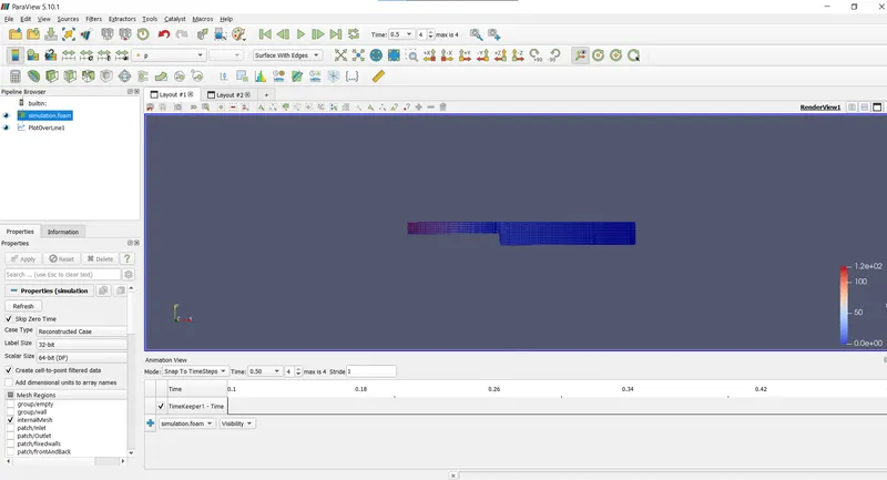
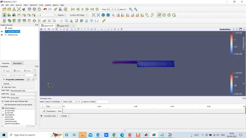
we will have to click on apply to view the boundary region.and then we will have to click on the suface with edges. so that we can see how the mesh is throughout the boundary.

Paraview :

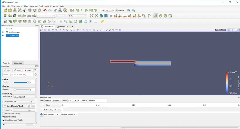
in paraview we will have click on apply option so that mesh will execute in the layout,it will appear in solid color,after we will have to go and select surface with edges option.since since we are trying to capture the velocity profile at 0.085,so that we will have to set the x axis dimensions to 0.085.and click on apply.after doing this we will be able to get the velocity profile at 0.085.click on plot over line command to select which profile we required based the question asked.in that we will have to selet the velocity so that we will be able to get the velocity graph.if we want to see that graph in another layout we can click on the addtion option and select line chart view.

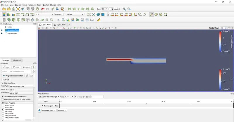
attaching profiles for grading factor 1 for 0.085 velocity from the inlet :

grading factor for 0.2 :

conclusion :

grading factor is defined as the ration between the width of the last cell of the domain to the width of the first cell of the domain.this factor works all the directions in the domain.

velocity and pressure curves are smoother where the grading factor in 1velocity and pressure curves are not smoother but its finer where the grading factor,so we can conlude to get the accurate results we will have to use the finer mesh.where the grading factor value is less there is high possibilities to get the accurate results since the cell size decreases.