Week 4.1 - Genetic Algorithm

AIM:

• Write a code in MATLAB to optimise the stalagmite function and find the global maxima of the function.
• Clearly expalin the concept of genetic algorithm in your own words and also explain the syntax for ga in MATLAB in report.
• Plot graphs for all 3 studies and for F maximum vs no. of iterations. Title and axes labels are a must, legends could be shown if necessary.

Introduction to Optimization

Optimization is the process of making something better. In any process, we have a set of inputs and a set of outputs as shown in the following figure.

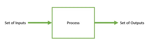
Optimization refers to finding the values of inputs in such a way that we get the “best” output values. The definition of “best” varies from problem to problem, but in mathematical terms, it refers to maximizing or minimizing one or more objective functions, by varying the input parameters.

The set of all possible solutions or values which the inputs can take make up the search space. In this search space, lies a point or a set of points which gives the optimal solution. The aim of optimization is to find that point or set of points in the search space.

What are Genetic Algorithms?

Genetic Algorithm (GA) is a search-based optimization technique based on the principles of Genetics and Natural Selection. It is frequently used to find optimal or near-optimal solutions to difficult problems which otherwise would take a lifetime to solve. It is frequently used to solve optimization problems, in research, and in machine learning.

Nature has always been a great source of inspiration to all mankind. Genetic Algorithms (GAs) are search based algorithms based on the concepts of natural selection and genetics. GAs are a subset of a much larger branch of computation known as Evolutionary Computation.

GAs were developed by John Holland and his students and colleagues at the University of Michigan, most notably David E. Goldberg and has since been tried on various optimization problems with a high degree of success.

In GAs, we have a pool or a population of possible solutions to the given problem. These solutions then undergo recombination and mutation (like in natural genetics), producing new children, and the process is repeated over various generations. Each individual (or candidate solution) is assigned a fitness value (based on its objective function value) and the fitter individuals are given a higher chance to mate and yield more “fitter” individuals. This is in line with the Darwinian Theory of “Survival of the Fittest”.

In this way we keep “evolving” better individuals or solutions over generations, till we reach a stopping criterion.

Genetic Algorithms are sufficiently randomized in nature, but they perform much better than random local search (in which we just try various random solutions, keeping track of the best so far), as they exploit historical information as well.

Basic Structure

We start with an initial population (which may be generated at random or seeded by other heuristics), select parents from this population for mating. Apply crossover and mutation operators on the parents to generate new off-springs. And finally these off-springs replace the existing individuals in the population and the process repeats. In this way genetic algorithms actually try to mimic the human evolution to some extent.

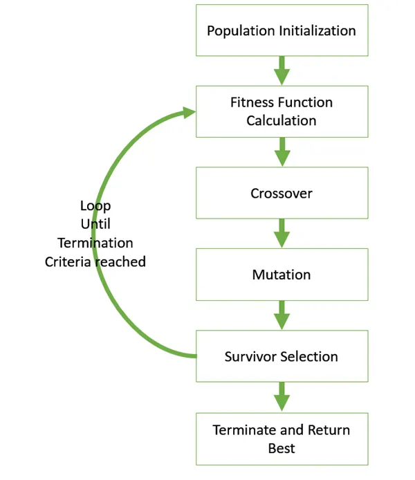
BASIC STRUCTURE:

GA()
   initialize population
   find fitness of population
   
   while (termination criteria is reached) do
      parent selection
      crossover with probability pc
      mutation with probability pm
      decode and fitness calculation
      survivor selection
      find best
   return best

Advantages of GAs

GAs have various advantages which have made them immensely popular. These include −

• Does not require any derivative information (which may not be available for many real-world problems).

• Is faster and more efficient as compared to the traditional methods.

• Has very good parallel capabilities.

• Optimizes both continuous and discrete functions and also multi-objective problems.

• Provides a list of “good” solutions and not just a single solution.

• Always gets an answer to the problem, which gets better over the time.

• Useful when the search space is very large and there are a large number of parameters involved.

Limitations of GAs

Like any technique, GAs also suffer from a few limitations. These include −

• GAs are not suited for all problems, especially problems which are simple and for which derivative information is available.

• Fitness value is calculated repeatedly which might be computationally expensive for some problems.

• Being stochastic, there are no guarantees on the optimality or the quality of the solution.

• If not implemented properly, the GA may not converge to the optimal solution.

GA APPLICATIONS:

Genetic Algorithms are primarily used in optimization problems of various kinds, but they are frequently used in other application areas as well.

In this section, we list some of the areas in which Genetic Algorithms are frequently used. These are −

• Optimization − Genetic Algorithms are most commonly used in optimization problems wherein we have to maximize or minimize a given objective function value under a given set of constraints. The approach to solve Optimization problems has been highlighted throughout the tutorial.

• Economics − GAs are also used to characterize various economic models like the cobweb model, game theory equilibrium resolution, asset pricing, etc.

• Neural Networks − GAs are also used to train neural networks, particularly recurrent neural networks.

• Parallelization − GAs also have very good parallel capabilities, and prove to be very effective means in solving certain problems, and also provide a good area for research.

• Image Processing − GAs are used for various digital image processing (DIP) tasks as well like dense pixel matching.

• Vehicle routing problems − With multiple soft time windows, multiple depots and a heterogeneous fleet.

• Scheduling applications − GAs are used to solve various scheduling problems as well, particularly the time tabling problem.

• Machine Learning − as already discussed, genetics based machine learning (GBML) is a niche area in machine learning.

• Robot Trajectory Generation − GAs have been used to plan the path which a robot arm takes by moving from one point to another.

• Parametric Design of Aircraft − GAs have been used to design aircrafts by varying the parameters and evolving better solutions.

• DNA Analysis − GAs have been used to determine the structure of DNA using spectrometric data about the sample.

• Multimodal Optimization − GAs are obviously very good approaches for multimodal optimization in which we have to find multiple optimum solutions.

• Traveling salesman problem and its applications − GAs have been used to solve the TSP, which is a well-known combinatorial problem using novel crossover and packing strategies.

GA INBUILT COMMAND OVERVIEW:

x = ga(fun,nvars,A,b,Aeq,beq,lb,ub,nonlcon,options)

fomula defines,

fun=given function,

nvars=number of variables

a,b,aeq,beq=these are used to if the equation(in our case we don't use because of the we do give the blanks in the place,

lb,ub=lower bounds &upper bounds[ include lower bound and upper bound values in this challenge we use this for 2nd and 3rd behavior of the function].

nonlcon=this represents linear & nonlinear equations

options=where we use to give the population size by using optimoptions command

STALAGMITE FUNCTION:

function [F]=stalagmite(input)

x=input(1);
y=input(2);

f1=(sin(5.1*pi*x+0.5))^6;
f2=(sin(5.1*pi*y+0.5))^6;
f3=exp((-4*log(2)*((x-0.0667)^2)/0.64));
f4=exp((-4*log(2)*((y-0.0667)^2)/0.64));

F=-(f1*f2*f3*f4);
end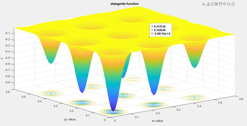

1rd case:unbounded statistical behaviour:

%statistical behavior of unbounded condition.
clear all
close all
clc

x=linspace(0,0.6,100);
y=linspace(0,0.6,100);
[xx, yy]=meshgrid(x,y);

for i=1:length(xx)
    for j =1:length(yy)
        input(1)=xx(i,j);                   
        input(2)=yy(i,j);
       f(i,j)=stalagmite(input);
    end
end

figure(1)
surfc(xx,yy,f,'LineWidth',3,'EdgeColor','flat')
xlabel('xx value')
ylabel('yy value')
zlabel('f')
shading interp
title('stalagmite function')

%statistical behavior of unbounded condition
tic
num_cases=50;
for i=1:num_cases
    [inputs,fopt(i)]=ga(@stalagmite,2);
    xopt(i)=inputs(1);
    yopt(i)=inputs(2);
    fopt(i)=-fopt(i)
end
study_time1=toc;

figure(2)
subplot(2,1,1);
hold on
surf(x,y,f);
plot3(xopt,yopt,fopt,'Marker','*','MarkerSize',3,'MarkerFaceColor','auto')
shading interp

subplot(2,1,2)
plot(fopt)
xlabel('iterations')
ylabel('maximum function value')
title('unbounded condition')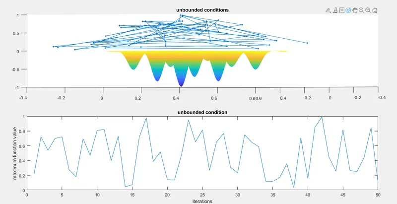

STUDY_TIME1=4.113843200000000

3rd case:increase iterations &define boundary limits

%statistical behavior of ga with bounded inputs
clear all
close all
clc

x=linspace(0,0.6,100);
y=linspace(0,0.6,100);
[xx, yy]=meshgrid(x,y);

for i=1:length(xx)
    for j =1:length(yy)
        input(1)=xx(i,j);                   
        input(2)=yy(i,j);
       f(i,j)=stalagmite(input);
    end
end

tic
num_cases=100;
for i=1:num_cases
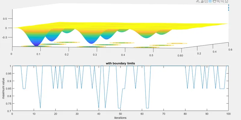
    [inputs,fopt(i)]=ga(@stalagmite,2,[],[],[],[],[0,0],[0.6,0.6]);
    xopt(i)=input(1);
    yopt(i)=input(2);
    fopt(i)=-fopt(i);
end
study_time2=toc;

figure(1)
subplot(2,1,1)
hold on
surfc(x,y,f)
plot3(xopt,yopt,fopt,'Marker','*','MarkerSize',3,'MarkerEdgeColor','auto')
shading interp
subplot(2,1,2)
plot(fopt)
xlabel('iterations')
ylabel('maximum value')
title('with boundary limits')

STUDY_TIME2=10.922457600000000

3rd case:increase iterations &inclde population size

%statistical behavior of ga with bounded inputs
%add the population size
clear all
close all
clc

x=linspace(0,0.6,100);
y=linspace(0,0.6,100);
[xx, yy]=meshgrid(x,y);

for i=1:length(xx)
    for j =1:length(yy)
        input(1)=xx(i,j);                   
        input(2)=yy(i,j);
       f(i,j)=stalagmite(input);
    end
end

tic
num_cases=150;
options=optimoptions('ga');
options=optimoptions(options,'PopulationSize',150);
for i=1:num_cases
    [inputs,fopt(i)]=ga(@stalagmite,2,[],[],[],[],[0,0],[0.6,0.6],[],options);
    xopt(i)=input(1);
    yopt(i)=input(2);
    fopt(i)=-fopt(i);
end
study_time3=toc;

figure(1)
subplot(2,1,1)
hold on
surfc(x,y,f)
plot3(xopt,yopt,fopt,'Marker','*','MarkerSize',3,'MarkerEdgeColor','auto')
shading interp
subplot(2,1,2)
plot(fopt)
xlabel('iterations')
ylabel('maximum value')
title('include pop size')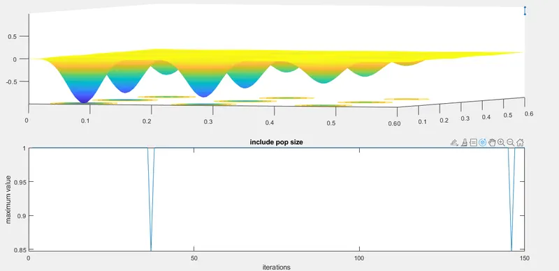

STUDY_TIME3=25.837216300000000

OVERVIEW OF THE RESULT:

if we observe the 3 ga graphs we were able to see the time it tooks to execute the function has different.this means if we increase the population size it takes much time to get the results.each and every we will get the different results while run the program because ga will not give us a same value each time.

the accurate values of the given function will be always depends on the population size.if we increase the population size there will be high chances of getting accurate results.but the same time it will take more time to get.we can clearly see the difference of the the 3 statistical behaviors of GA .

scripting procedure wih the commands:

• clear all,close all clc these aere the commands were used to clear all the exist outputs,exist scripts and fresh page of command window.
• define required no.of x & y values by using linspace command.
• to convert that 1d array of x&y to 2d we use meshgrid command.it helps to convert all the 1d arrays to 2d.
• creat a function script of the given function,named it as stlagmite which contain 2 variables.
• and find out the variables and include that variable into the stalagmite function by using for loop. which will give us a stalagmite shaped graph which is shown above.
• tic &toc command is used to find out the time period of each statistical behavior of ga
• ga is an inbuilt command which is always used to find out the minimun value of the function.ga command is deeply explained above.
• we have given num_cases vary to each behavior for executing more number of times we use for loop again.
• subplot is the command used to get the graph in a required no.of columns &rows
• surf is command is used to get the 2d arrays is 3d view.
• plot3 is the command is used to get the 3 coordinates graph in one figure
• hold on command is used to get the no of graphs in same figure.
• shading interp is the command is used to get the smooth curve without appearing any type of grids.
• xlabel &ylabel is used give the names of the axis
• title command is used to give the the name of the final result or what the graph defines.

• WE HAVE TO FIND THE MAXIMUM VALUE OF THE GIVEN FUNCTION IN THIS PROJECT,BUT GA ALWAYS FIND THE MINIMUM VALUE OF THE FUNCTION FOR THE WE USE TO REVERSING THE GIVEN FUNCTION WE WERE ABLE TO GET THE MAXIMUM VALUE. FOR THAT PURPOSE WE HAVE GIVE '-' sign TO THE FUNCTION AFTER EXECUTING GA.

REFERENCES:

1)MATHWORKS OFFICIAL WEBSITE

2)WIKIPEDIA OF GA

3)TOOK REFERENCE OF SOME YOUTUBE VIDEOS

4)SKILL LYNC WEB PAGE & SUPPORT ENGINEER GUIDANCE

5)APPLICATION ON TUTORIALS POINT