Week 3.5 - Deriving 4th order approximation of a 2nd order derivative using Taylor Table method
aim :
Derive the following 4th order approximations of the second-order derivative. Central difference,. Skewed right-sided difference, Skewed left-sided difference and show the grpah which one in is give exact values
objectve :
- to paste the code and explain the output values
- Write a detailed explanation for results.explain the Plots and codes
- we have to find out the all the three approximation formulas by using given hints.
4th order forward skewed difference approximation for the 2nd derivative of the given function :
`Deltax^2(partial^2f)/(partialx^2)=a*f(x)+b*f(x+dx)+c*f(x+2dx)+d*f(x+3dx)+e*f(x+4dx)+g*f(x+5dx)`
`a*f(x)=a*f(x)`
`b*f(x+Deltax)=b[f(x)+f'(Deltax)+f''((Deltax^2)/2)+f'''((Deltax^3)/6)+f''''((Deltax^4)/24)+f'''''((Deltax^5)/120)]`
`c*f(x+2Deltax)=c[f(x)+f'(2Deltax)+f''((4Deltax^2)/2)+f'''((8Deltax^3)/6)+f''''((16Deltax^4)/24)+f'''''((32Deltax^5)]/120)]`
`d*f(x+3Deltax)=d[f(x)+f'(3Deltax)+f''((9Deltax^2)/2)+f'''((27Deltax^3)/6)+f''''((81Deltax^4)/24)+f'''''((243Deltax^5)]/120)]`
`e*f(x+4Deltax)=e[f(x)+f'(4Deltax)+f''((16Deltax^2)/2)+f'''((64Deltax^3)/6)+f''''((256Deltax^4)/24)+f'''''((1024Deltax^5)]/120)]`
`g*f(x+5Deltax)=g[f(x)+f'(5Deltax)+f''((25Deltax^2)/2)+f'''((125Deltax^3)/6)+f''''((625Deltax^4)/24)+f'''''((3125Deltax^5)]/120)]`
| `f(x)` | `Deltax*f'(x)` | `Deltax^2*f''(x)` | `Deltax^3*f'''(x)` | `Deltax^4*f''''(x)` | `Deltax^5*f'''''(x)` | ||||||||||||||||||||||||||||||||||||||||||||||||
| `af(x)` | a | 0 | 0 | 0 | 0 | 0 | |||||||||||||||||||||||||||||||||||||||||||||||
| `b*f(x+Deltax)` | b | b | b/2 | b/6 | b/24 | b/120 | |||||||||||||||||||||||||||||||||||||||||||||||
| `c*f(x+2Deltax)` | c | 2*c | 4*c/2 | 8*c/6 | 16*c/24 | 32*c/120 | |||||||||||||||||||||||||||||||||||||||||||||||
| `d*f(x+3Deltax)` | d | 3*d | 9*d/2 | 27*d/6 | 81*d/24 | 243*d/120 | |||||||||||||||||||||||||||||||||||||||||||||||
| `e*f(x+4Deltax)` | e | 4*e | 16e/2 | 64e/6 | 256e/24 | 1024*e/120 | |||||||||||||||||||||||||||||||||||||||||||||||
| `g*f(x+5Deltax)` | g | 5*g | 25g/2 | 125g/6 | 625g/24 | 3125g/120 | |||||||||||||||||||||||||||||||||||||||||||||||
| co-effs comp LHS | 0 | 0 | 1 | 0 | 0 | 0 |
compare the coefficients on both the sides :
the equation we get is
`(a+b+c+d+e+g)f(x)=0`
`(0+b+2c+3d+4e+5g)f'(x)=0`
`(0+b/2+(4c)/2+(9d)/2+(16e)/2+(25g)/2)f''(x)=1`
`(0+b/6+(8c)/6+(27d)/6+(64e)/6+(125g)/6)f'''(x)=0`
`(0+b/24+(16c)/24+(81d)/24+(256e)/24+(625g)/24)f''''(x)=0`
`(0+b/120+(16c)/120+(81d)1/20+(256e)/120+(625g)/120)f'''''(x)=0`
we can easily find out the coefficient values if we convers the above eq's into a matrix form :
A =`[[1,1,1,1,1,1],[0,1,2,3,4,5],[0,1/2,4/2,9/2,16/2,25/2],[0,1/6,8/6,27/6,64/6,125/6],[0,1/24,16/24,81/24,256/24,625/24],[0,1/120,32/120,243/120,1024/120,3125/120]]`
X=`((a),(b),(c),(d),(e),(g))`
B=`((0),(0),(1),(0),(0),(0))`
matrix in the form of AX=B
`X=A^-1*B`
X=`((a),(b),(c),(d),(e),(g))`=`(( 3.7500),(-12.8333 ), (17.8333),( -13.0000),( 5.0833) ,( -0.8333))`
WE WILL BE ABLE TO FIND OUT THE EQUATION bu using above formula.
how to define the no.of nodes :
for both skewed forward and backward difference approximation we use
number of nodes=p+q
p=order of the approximation(4) ;q=order of the derivative(2);
then p+q=2+4=6
conclusion : we have to find upto 6 nodes for 2nd derivative of the 4th order approximation both forward &backward skewed difference approximation.
4th order backward skewed difference approximation for the 2nd derivative of the given function :
`Deltax^2*(partial^2f)/(partialx^2)=a*f(x)+b*f(x-dx)+c*f(x-2dx)+d*f(x-3dx)+e*f(x-4dx)+g*f(x-5dx)`
`a*f(x)=a*f(x)`
`b*f(x-Deltax)=b[f(x)-f'(Deltax)+f''((Deltax^2)/2)-f'''((Deltax^3)/6)+f''''((Deltax^4)/24)-f'''''((Deltax^5)/120)]`
`c*f(x-2Deltax)=c[f(x)-f'(2Deltax)+f''((4Deltax^2)/2)-f'''((8Deltax^3)/6)+f''''((16Deltax^4)/24)-f'''''((32Deltax^5)]/120)]`
`d*f(x-3Deltax)=d[f(x)-f'(3Deltax)+f''((9Deltax^2)/2)-f'''((27Deltax^3)/6)+f''''((81Deltax^4)/24)-f'''''((243Deltax^5)]/120)]`
`e*f(x-4Deltax)=e[f(x)-f'(4Deltax)+f''((16Deltax^2)/2)-f'''((64Deltax^3)/6)+f''''((256Deltax^4)/24)-f'''''((1024Deltax^5)]/120)]`
`g*f(x-5Deltax)=g[f(x)-f'(5Deltax)+f''((25Deltax^2)/2)-f'''((125Deltax^3)/6)+f''''((625Deltax^4)/24)-f'''''((3125Deltax^5)]/120)]`
| `f(x)` | `Deltax*f'(x)` | `Deltax^2*f''(x)` | `Deltax^3*f'''(x)` | `Deltax^4*f''''(x)` | `Deltax^5*f'''''(x)` | ||||||||||||||||||||||||||||||||||||||||||||||||
| `af(x)` | a | - 0 | 0 | - 0 | 0 | - 0 | |||||||||||||||||||||||||||||||||||||||||||||||
| `b*f(x-Deltax)` | b | - b | b/2 | -b/6 | b/24 | - b/120 | |||||||||||||||||||||||||||||||||||||||||||||||
| `c*f(x-2Deltax)` | c | -2*c | 4*c/2 | -8*c/6 | 16*c/24 | - 32*c/120 | |||||||||||||||||||||||||||||||||||||||||||||||
| `d*f(x-3Deltax)` | d | - 3*d | 9*d/2 | -27*d/6 | 81*d/24 | - 243*d/120 | |||||||||||||||||||||||||||||||||||||||||||||||
| `e*f(x-4Deltax)` | e | -4*e | 16e/2 | -64e/6 | 256e/24 | -1024*e/120 | |||||||||||||||||||||||||||||||||||||||||||||||
| `g*f(x-5Deltax)` | g | - 5*g | 25g/2 | -125g/6 | 625g/24 | -3125g/120 | |||||||||||||||||||||||||||||||||||||||||||||||
| co-effs comp LHS | 0 | 0 | 1 | 0 | 0 | 0 |
compare the coefficients on both the sides :
the equation we get is
`(a+b+c+d+e+g)f(x)=0`
`(0-b-2c-3d-4e-5g)f'(x)=0`
`(0+b/2+(4c)/2+(9d)/2+(16e)/2+(25g)/2)f''(x)=1`
`(0-b/6-(8c)/6-(27d)/6-(64e)/6-(125g)/6)f'''(x)=0`
`(0+b/24+(16c)/24+(81d)/24+(256e)/24+(625g)/24)f''''(x)=0`
`(0-b/120-(16c)/120-(81d)/20-(256e)/120-(625g)/120)f'''''(x)=0`
we can easily find out the coefficient values if we convers the above eq's into a matrix form :
A =`[[1,1,1,1,1,1],[-0,-1,-2,-3,-4,-5],[0,1/2,4/2,9/2,16/2,25/2],[-0,-1/6,-8/6,-27/6,-64/6,-125/6],[0,1/24,16/24,81/24,256/24,625/24],[-0,-1/120,-32/120,-243/120,-1024/120,-3125/120]]`
X=`((a),(b),(c),(d),(e),(g))`
B=`((0),(0),(1),(0),(0),(0))`
matrix in the form of AX=B
`X=A^-1*B`
X=`((a),(b),(c),(d),(e),(g))`=`((3.7500),( -12.8333),( 17.8333), (-13.0000),( 5.0833 ), ( -0.8333))`
WE WILL BE ABLE TO FIND OUT THE EQUATION bu using above formula.
how to define the no.of nodes :
for both skewed forward and backward difference approximation we use
number of nodes=p+q
p=order of the approximation(4) ;q=order of the derivative(2);
then p+q=2+4=6
conclusion : we have to find upto 6 nodes for 2nd derivative of the 4th order approximation both forward &backward skewed difference approximation.
4th order central difference approximation or symmetric for the 2nd derivative of the given function :
`Deltax^2*(partial^2f)/(partialx^2)=a*f(x-2dx)+b*f(x-dx)+c*f(x)+d*f(x+dx)+e*f(x+2dx)`
`a*f(x-2Deltax)=a[f(x)-f'(2Deltax)+f''((4Deltax^2)/2)-f'''((8Deltax^3)/6)+f''''((16Deltax^4)/24)-f'''''((32Deltax^5)]/120)]`
`b*f(x-Deltax)=b[f(x)-f'(Deltax)+f''((Deltax^2)/2)-f'''((Deltax^3)/6)+f''''((Deltax^4)/24)-f'''''((Deltax^5)/120)]`
`c*f(x)=c*f(x)`
`d*f(x+Deltax)=d[f(x)+f'(Deltax)+f''((Deltax^2)/2)+f'''((Deltax^3)/6)+f''''((Deltax^4)/24)+f'''''((Deltax^5)/120)]`
`e*f(x+2Deltax)=e[f(x)+f'(2Deltax)+f''((4Deltax^2)/2)+f'''((8Deltax^3)/6)+f''''((16Deltax^4)/24)+f'''''((32Deltax^5)]/120)]`
| `f(x)` | `Deltax*f'(x)` | `Deltax^2*f''(x)` | `Deltax^3*f'''(x)` | `Deltax^4*f''''(x)` | ||||||||||||||||||||||||||||||||||||||||||||
| `a*f(x-2Deltax)` | a | - 2a | 4a/2 | -8a/2 | 16a/24 | |||||||||||||||||||||||||||||||||||||||||||
| `b*f(x-Deltax)` | b | - b | b/2 | -b/6 | b/24 | |||||||||||||||||||||||||||||||||||||||||||
| `c*f(x)` | c | 0 | 0 | 0 | 0 | |||||||||||||||||||||||||||||||||||||||||||
| `d*f(x+Deltax)` | d | d | d/2 | d/6 | d/24 | |||||||||||||||||||||||||||||||||||||||||||
| `e*f(x+2Deltax)` | e | 2*e | 4e/2 | 8e/6 | 16e/24 | |||||||||||||||||||||||||||||||||||||||||||
| co-effs comp LHS | 0 | 0 | 1 | 0 | 0 |
compare the coefficients on both the sides :
the equation we get is
`(a+b+c+d+e)f(x)=0`
`(-2a-b+0+d+2e)f'(x)=0`
`((4a)/2+b/2+0+d/2+(4e)/2)f''(x)=1`
`((-8a)/6-b/6+0+d/6+(8e)/6)f'''(x)=0`
`((16a)/24+b/24+0+d/24+(16e)/24)f''''(x)=0`
we can easily find out the coefficient values if we convers the above eq's into a matrix form :
A =`[[1,1,1,1,1],[-2,-1,0,1,2],[2,1/2,0,1/2,2],[-8/6,-1/6,0,1/6,8/6],[16/24,1/24,0,1/24,16/24]]`
X=`((a),(b),(c),(d),(e))`
B=`((0),(0),(1),(0),(0))`
matrix in the form of AX=B
`X=A^-1*B`
X= `((a),(b),(c),(d),(e))`=`((-0.0833),( 1.3333), (-2.5000) ,(1.3333) ,(-0.0833))`
WE WILL BE ABLE TO FIND OUT THE EQUATION bu using above formula.
how to define the no.of nodes & the coefficients to find:
for central difference approximation we use
number of nodes=p+q-1
p=order of the approximation(4) ;q=order of the derivative(2);
then p+q=2+4-1=5
conclusion : we have to find upto 5 nodes for 2nd derivative of the 4th order approximation central difference approximation.
we have rewrite the equations here ;
skewed forward difference approximation :
`(partial^2f)/(partialx^2)=(a*f(x)+b*f(x+dx)+c*f(x+2dx)+d*f(x+3dx)+e*f(x+4dx)+g*f(x+5dx))/(Deltax^2)``
skewed backward difference approximation :
`(partial^2f)/(partialx^2)=(a*f(x)+b*f(x-dx)+c*f(x-2dx)+d*f(x-3dx)+e*f(x-4dx)+g*f(x-5dx))/(Deltax^2)`
central difference approximation :
`(partial^2f)/(partialx^2)=(a*f(x-2dx)+b*f(x-dx)+c*f(x)+d*f(x+dx)+e*f(x+2dx))/(Deltax^2)`
programmimg part :
main script :
clear all
close all
clc
 x=pi/3;
 dx=linspace(pi/3,pi/3000,20);

%given function f(x)=exp(x)*cos(x)
         % f'(x)=exp(x*)cos(x)-exp(x)*sin(x)
         % f''(x)=-2*exp(x)*sin(x)

%skewed f.d.a coefficients
A_fda =[1,1,1,1,1,1;0,1,2,3,4,5;0,1/2,4/2,9/2,16/2,25/2;0,1/6,8/6,27/6,64/6,125/6; 0,1/24,16/24,81/24,256/24,625/24;0,1/120,32/120,243/120,1024/120,3125/120];
X_fda =['a';'b';'c';'d';'e';'g'];
B_fda=[0;0;1;0;0;0];
X_fda=A_fda^-1*B_fda;
a_fda=X_fda(1);
b_fda=X_fda(2);
c_fda=X_fda(3);
d_fda=X_fda(4);
e_fda=X_fda(5);
g_fda=X_fda(6);


%skewed b.d.a coefficients
A_bda =[1,1,1,1,1,1;-0,-1,-2,-3,-4,-5;0,1/2,4/2,9/2,16/2,25/2;-0,-1/6,-8/6,-27/6,-64/6,-125/6;0,1/24,16/24,81/24,256/24,625/24;-0,-1/120,-32/120,-243/120,-1024/120,-3125/120];
X_bda =['a';'b';'c';'d';'e';'g'];
B_bda=[0;0;1;0;0;0];
X_bda=A_bda^-1*B_bda;
a_bda=X_bda(1);
b_bda=X_bda(2);
c_bda=X_bda(3);
d_bda=X_bda(4);
e_bda=X_bda(5);
g_bda=X_bda(6);

%C.D.A coefficients
A_cda =([1,1,1,1,1;-2,-1,0,1,2;2,1/2,0,1/2,2;-8/6,-1/6,0,1/6,8/6;16/24,1/24,0,1/24,16/24]);
X_cda =['a';'b';'c';'d';'e'];
B_cda=[0;0;1;0;0];
%AX=B
X_cda=A_cda^-1*B_cda;
a_cda=X_cda(1);
b_cda=X_cda(2);
c_cda=X_cda(3);
d_cda=X_cda(4);
e_cda=X_cda(5);


for i=1:length(dx)
     [fda_error(i)]=error_fda(x,dx(i),a_fda,b_fda,c_fda,d_fda,e_fda,g_fda);
      [bda_error(i)]=error_bda(x,dx(i),a_bda,b_bda,c_bda,d_bda,e_bda,g_bda);
       [cda_error(i)]=error_cda(x,dx(i),a_cda,b_cda,c_cda,d_cda,e_cda);
end
mkdir('2nd derivative')
cd('2nd derivative')
figure(1)
loglog(dx,fda_error,'LineWidth',2,'Color','g')
hold on
loglog(dx,bda_error,'LineWidth',2,'Color','r')
hold on
loglog(dx,cda_error,'LineWidth',2,'Color','black')
hold off
xlabel('dx')
ylabel('errors')
legend('skewed fda error','skewed bda error','skewed cda error')
title('graph to show the errors with dx')

saveas(1,'errors','png')
cd ..
functions of all the three :
function [fda_error]=error_fda(x,dx,a_fda,b_fda,c_fda,d_fda,e_fda,g_fda)
%given function f(x)=exp(x)*cos(x)
         % f'(x)=e^x*cos(x)-e^x*sin(x)
         % f''(x)=-2*e^x*sin(x)
%analytical derivative
   analytical_derivative=-2*exp(x)*sin(x);

 %numerical deivative
 %4th order skewed forward difference approximation of 2nd derivative
skewed_fda =(a_fda*exp(x)*cos(x)+b_fda*(exp(x+dx)*cos(x+dx))+c_fda*(exp(x+2*dx)*cos(x+2*dx))+d_fda*(exp(x+3*dx)*cos(x+3*dx))+e_fda*(exp(x+4*dx)*cos(x+4*dx))+g_fda*(exp(x+5*dx)*cos(x+5*dx)))/(dx^2);
fda_error=abs(skewed_fda-analytical_derivative);
end
function [bda_error]=error_bda(x,dx,a_bda,b_bda,c_bda,d_bda,e_bda,g_bda)
%given function f(x)=exp(x)*cos(x)
% f'(x)=e^x*cos(x)-e^x*sin(x)
% f''(x)=-2*e^x*sin(x)
%analytical derivative
analytical_derivative=-2*exp(x)*sin(x);
%numerical deivative
%4th order skewed forward difference approximation of 2nd derivative
skewed_bda=(a_bda*(exp(x)*cos(x))+b_bda*(exp(x-dx)*cos(x-dx))+c_bda*(exp(x-2*dx)*cos(x-2*dx))+d_bda*(exp(x-3*dx)*cos(x-3*dx))+e_bda*(exp(x-4*dx)*cos(x-4*dx))+g_bda*(exp(x-5*dx)*cos(x-5*dx)))/(dx^2);
bda_error=abs(skewed_bda-analytical_derivative);
endfunction [cda_error]=error_cda(x,dx,a_cda,b_cda,c_cda,d_cda,e_cda)
%given function f(x)=exp(x)*cos(x)
% f'(x)=e^x*cos(x)-e^x*sin(x)
% f''(x)=-2*e^x*sin(x)
%analytical derivative
analytical_derivative=-2*exp(x)*sin(x);
%numerical deivative
%4th order skewed forward difference approximation of 2nd derivative
skewed_cda=((a_cda*(exp(x-2*dx))*cos(x-2*dx))+b_cda*(exp(x-dx)*cos(x-dx))+c_cda*(exp(x)*cos(x))+d_cda*(exp(x+dx)*cos(x+dx))+e_cda*(exp(x+2*dx)*cos(x+2*dx)))/(dx^2);
cda_error=abs(skewed_cda-analytical_derivative);
endcode explantion:
the process of finding the coefficients and finding the hypothesis equation for all the three methods has been explained above.
everything as per the same what we did in the last challange once we complete to find all the coefficient values and the hypothesis equation.we will have to define the x,dx values since dx is an array we have to use for loop here.i have created a individual function for all the three approximations.and call all the three functions into main script inside the for loop since we are using using length of dx and the dx is an array.
inside the function we have to find out the analytical values of the given function and substacting that analytical value to the approximation values which will give us how much error is occuring between those analytical and numeric values.
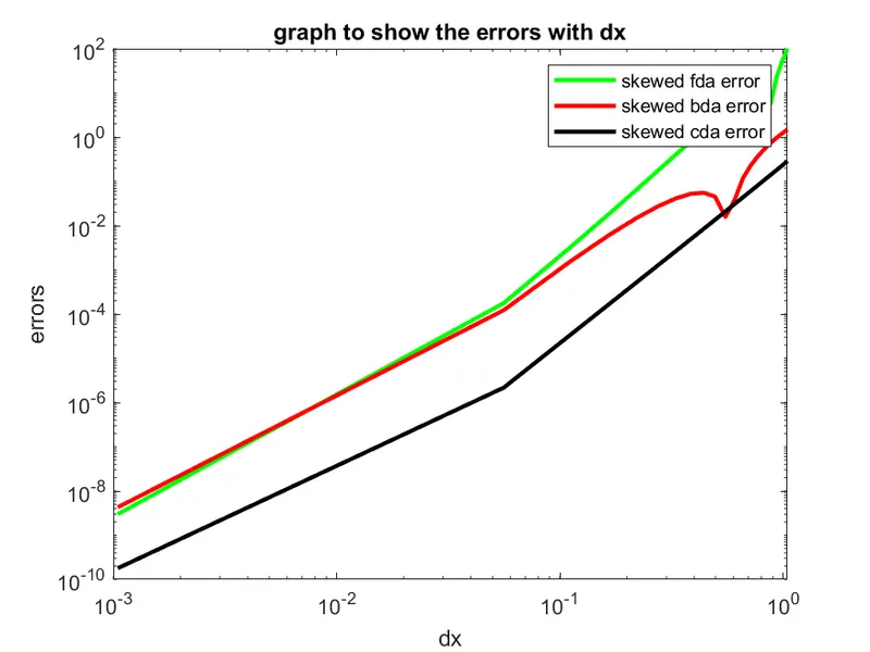
finally plot the errors of all the three aproximation arrors with respect to the dx values it shows how the three approximations varies w.r.to the dx values
save the plot using mkdir,cd,cd .. commands by creating the directory.
plot :
conclusion :
skewed both forward backward difference approximation is used to get the near possible results since we are trying to find out the near approximation values of each derivative.while central difference approximation is used to get the exact values of the given function because we were find by using all of its neighbouring points both the right and left so we will get the exact values.
the above statement is satisfied if we see the graph
graph observation : as we observe the graph we can see that the forward difference approximation error is producing high errors and dx range also increasing simoultaneosly &the backward difference order error is producing small errors and dx range also decreasing simoultaneosly . and finally the central difference approximation producing very lass error when compared to other two methods.in forward difference approximation error we can observe the starting point shows a best results of the approximation and finally its not giving us a possible exact value for the given information.in bacward difference approximation giving best results when compared to the last one .in central difference approximation error we can observe we are getting a large error at starting and finaly it is reducing the error towards the origin and also reducing the range of dx.sincecentral difference approximation error drastically changes its error values towards the exact solution we consider the central diff approx is the one we should use to get the exact value with minium error when compared to its last two methods.
we will have keep in mind always decide the method based on in which direction information is passing based on that we choose the method of approximation.