Week 8 - Simulation of a backward facing step in OpenFOAM

OBJECTIVE.

• To simulate an incompressible-laminar-viscous flow through the backwards-facing step geometry and perform a transient simulation.

• Case 1 - To Simulate the flow without using any grading factor (i.e., GF = 1)

  Case 2 - To Simulate the flow with a grading factor of 0.2. The cells should be finer near the walls (including the step wall).

Incompressible-laminar-viscous flow.

incompressible flow:

The flow in which there is no change in the density is called the incompressible flow.

Mathematically, an incompressible flow can be expressed as

Laminar flow:

A laminar flow is one where the fluid motion is regular and there is no mixing. It can be visualized by the pathlines that do not intersect each other.

In fluid dynamics, laminar flow is characterized by fluid particles following smooth paths in layers, with each layer moving smoothly past the adjacent layers with little or no mixing.

At low velocities, the fluid tends to flow without lateral mixing, and adjacent layers slide past one another like playing cards. There are no cross-currents perpendicular to the direction of flow, nor eddies or swirls of fluids.

In laminar flow, the motion of the particles of the fluid is very orderly with particles close to a solid surface moving in straight lines parallel to that surface. Laminar flow is a flow regime characterized by high momentum diffusion and low momentum convection.

Reynolds number is the parameter to differentiate a flow as laminar or turbulent.

Whenever the Reynolds number is less than about 2,000, flow in a pipe is generally laminar, whereas, at values greater than 2,000, flow is usually turbulent.

Mathematically, Reynolds number is the ratio of inertial force to the viscous force.

where,

• ρ is the density of the fluid (kg/m³)
• u is the flow speed (m/s)
• L is a characteristic linear dimension (m)
• μ is the dynamic viscosity of the fluid (Pa·s or N·s/m² or kg/(m·s))
• ν is the kinematic viscosity of the fluid (m²/s)

Viscous flow.

A type of fluid flow in which there is a continuous steady motion of the particles; the motion at a fixed point always remains constant. Also called streamline flow; laminar flow; steady flow.

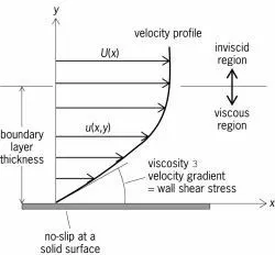
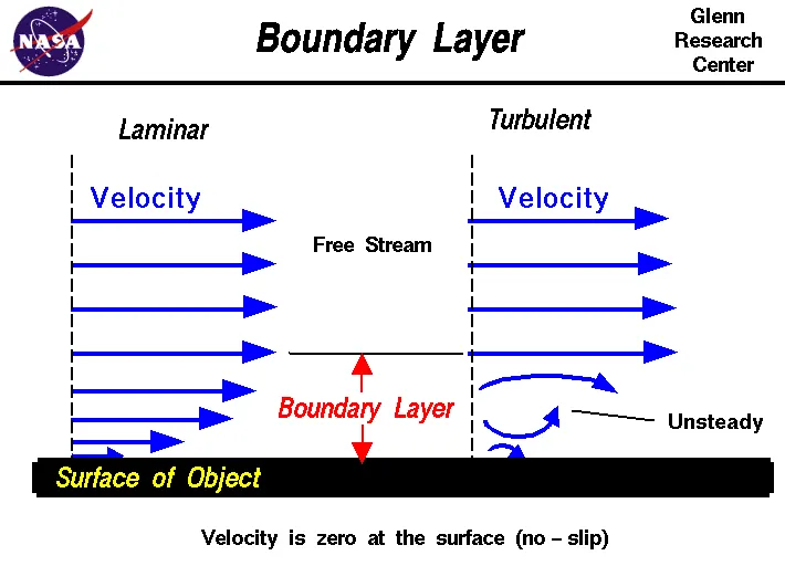
The fluid flow in form of a layer. The layer which sticks with the wall has zero velocity which is called no-slip condition and it develops the frictional effect at the wall. Frictional effects are also present between two layers of fluid and slower layer tries to slow down the faster layer which can be measured by using viscosity.

effects of viscosity are maximum near the boundary so laminar sublayer exists near the boundary that is shown in the below figure.

Mesh grading.

Mesh grading is a factor that is,

Grading factor = Size of the last cell / size of the first cell

PROCEDURE.

/*--------------------------------*- C++ -*----------------------------------*\
  =========                 |
  \\      /  F ield         | OpenFOAM: The Open Source CFD Toolbox
   \\    /   O peration     | Website:  https://openfoam.org
    \\  /    A nd           | Version:  9
     \\/     M anipulation  |
\*---------------------------------------------------------------------------*/
FoamFile
{
    format      ascii;
    class       dictionary;
    object      blockMeshDict;
}
// * * * * * * * * * * * * * * * * * * * * * * * * * * * * * * * * * * * * * //

convertToMeters 0.01;

vertices
(
    (0 0 0) // vertex 0
    (8 0 0) // vertex 1
    (8 0.5 0) // vertex 2
    (0 0.5 0) // vertex 3
    (8 1 0) // vertex 4
    (0 1 0) //   vertex 5
    (20 1 0) // vertex 6
    (20 0.5 0) // vertex 7
    (20 0 0) // vertex 8
    (20 -1 0) // vertex 9
    (8 -1 0) // vertex 10
    (0 0 1) // vertex 11
    (8 0 1) // vertex 12
    (8 0.5 1) // vertex 13
    (0 0.5 1) // vertex 14
    (8 1 1) // vertex 15
    (0 1 1) // vertex 16
    (20 1 1) // vertex 17
    (20 0.5 1) // vertex 18
    (20 0 1) // vertex 19
    (20 -1 1) // vertex 20
    (8 -1 1) // vertex 21
    
);

blocks
(
    hex (0 1 2 3 11 12 13 14) (50 5 1) simpleGrading (1 5 1)
    hex (3 2 4 5 14 13 15 16) (50 5 1) simpleGrading (1 0.2 1)
    hex (2 7 6 4 13 18 17 15) (150 5 1) simpleGrading (5 0.2 1)
    hex (1 8 7 2 12 19 18 13) (150 5 1) simpleGrading (5 5 1)
    hex (10 9 8 1 21 20 19 12) (150 20 1) simpleGrading (5 10 1)
);

edges
(
);

boundary
(
    inlet
    {
        type patch;
        faces
        (
            (0 11 14 3) // Patch 1
            (3 14 16 5) // Patch 2
        );
    }
    outlet
    {
        type patch;
        faces
        (
            (9 8 19 20) // Patch 1
            (8 7 18 19) // Patch 2
            (7 6 17 18) // Patch 3
        );
    }
    walls
    {
        type wall;
        faces
        (
            (4 5 16 15) // wall 1 (upward -left)
            (6 4 15 17) // wall 2 (upward -right)
            (0 1 12 11) // wall 3 (downward -left)
            (10 9 20 21) // wall 4 (downward -right)
            (10 21 12 1) // Outward normal flow towards right
            
        );
    } 
    frontAndBack
    {
        type empty;
        faces
        (
            (0 3 2 1) // Back wall 1 
            (3 5 4 2) // Back wall 2 
            (10 1 8 9) // Back wall 3 
            (1 2 7 8) // Back wall 4 
            (2 4 6 7) // Back wall 5 
            (11 14 13 12) // Front wall 1 
            (14 16 15 13) // Front wall 2 
            (21 12 19 20) // Front wall 3 
            (12 13 18 19) // Front wall 4 
            (13 15 17 18) // Front wall 5 
            
        );
    } 
);

mergePatchPairs
(
);

// ************************************************************************* //

/*--------------------------------*- C++ -*----------------------------------*\
  =========                 |
  \\      /  F ield         | OpenFOAM: The Open Source CFD Toolbox
   \\    /   O peration     | Website:  https://openfoam.org
    \\  /    A nd           | Version:  9
     \\/     M anipulation  |
\*---------------------------------------------------------------------------*/
FoamFile
{
    format      ascii;
    class       dictionary;
    location    "system";
    object      controlDict;
}
// * * * * * * * * * * * * * * * * * * * * * * * * * * * * * * * * * * * * * //

application     icoFoam;

startFrom       startTime;

startTime       0;

stopAt          endTime;

endTime         20;

deltaT          1e-2;

writeControl    timeStep;

writeInterval   20;

purgeWrite      0;

writeFormat     ascii;

writePrecision  6;

writeCompression off;

timeFormat      general;

timePrecision   6;

runTimeModifiable true;


// ************************************************************************* //

• First, we are creating the run folder in OpenFOAM in which we will be running our simulations.
• And then need to copy the cavity folder to the run folder so that we can make the changes in the blockMeshDict, controlDict, and pressure and velocity files as to run our required simulations, we copying the folder because we are not supposed to make any changes in the original folders in the OpenFOAM.
• Then will make the required changes in the blockMeshDict file that is naming the vertices for and then creating the blocks, in this case, there are 21 vertices and 5 blocks while creating blocks we also need to specify the number of mesh points needed along the x, y, and z-direction and also the simple grading should be done along the boundaries.
• then, we need to assign the boundary conditions here, we need to define all the faces in OpenFOAM refers to patches and giving them type that is the inlet and outlet will be the faces (type patch), for front and back type will be empty faces, for top and bottom which are the boundary conditions in this case type will be wall type and setting up these will constitute a particular boundary, then will save these changes in the blockMeshDict.
• Then, in the velocity and pressure files, we have to give the value of the velocity at the inlet type will be fixed value here we should assign some value as initial velocity and pressure will be zerogradient and at the outlet velocity type will be zerogradient and pressure will be type fixedvalue that value will be uniform 0, then at front and back velocity type empty and pressure, as well as type empty at the no slip boundaries that is top and bottom velocity, will be type noslip and pressure type empty. And in the transportProperties we can change the nu value in order to obtain the lower courant number.
• And in the controlDict file the simulation time and the time step need be assigned in the way that the courant number should be less than 0.5.
• and then creating the block mesh and then run the simulation using the respective solver after the completion of simulation open the paraview in the paraFoam and plot the velocity profile for the given value.

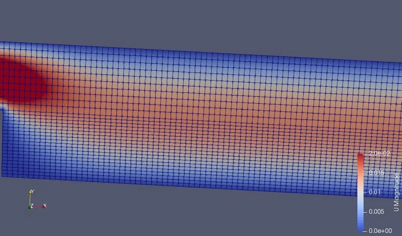
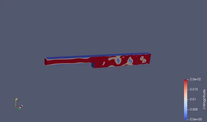
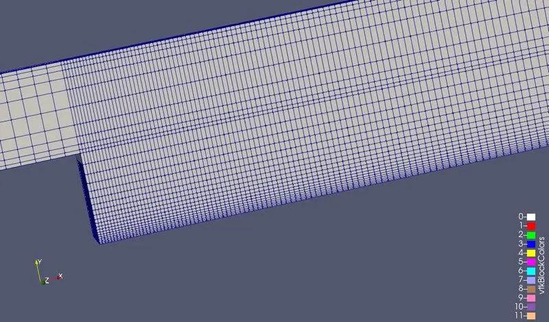
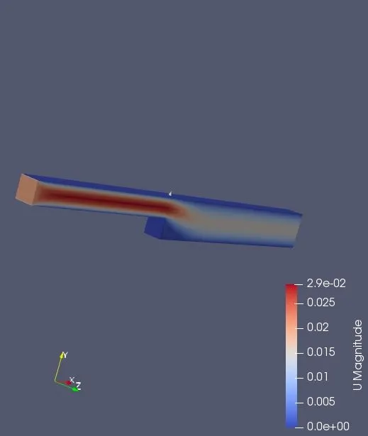
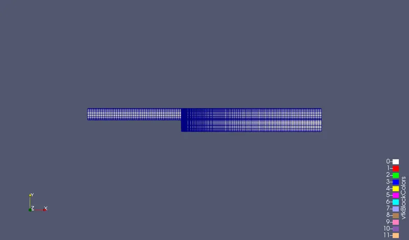
Mesh size is refined near the area of cross section where flow might get unstable due to geometry variation by a step size of 0.01,

made finer to coarser on the 0.12 m plate area.

RESULT :

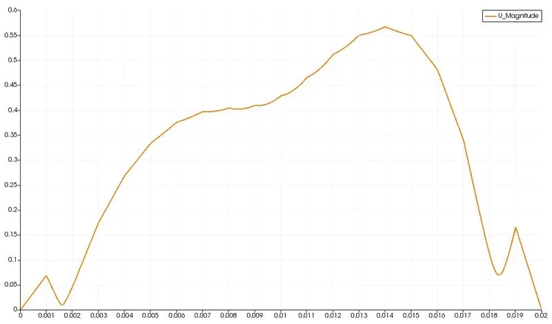
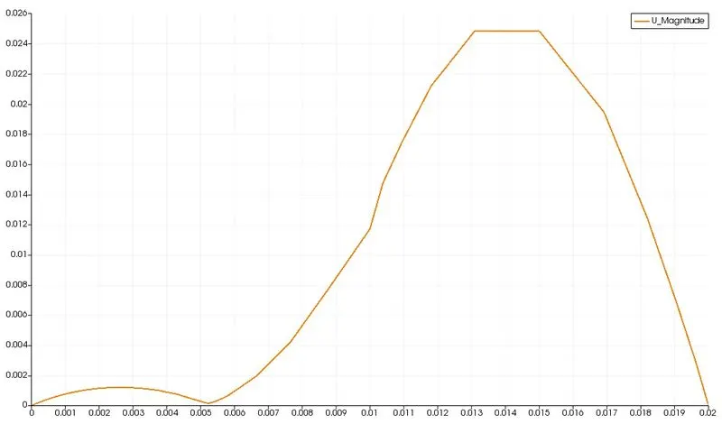
- Up to this point, we have done plotting velocity plot for both, without grading factor and with 0.2 grading factor, cases. If we take a look at all the three line graph, we can see, the plot for velocity without grading factor seems more smooth and accurate than other two plot. So one can say, grading can disrupt out result. But it is incorrect. Because, if we take good look at it, we can notice, the mesh is fine at step wall along the X-axis but very coarse along Y-axis. Therefore, we are not getting smooth plot for velocity at 0.085 point at Y-axis.

- We obtain results for an equally spaced simple grading and a fine to coarse ratio simple grading.

- To understand this thing clearly, we can see below figure, where we can see- on the left side there is coarse mesh and on the right side fine mesh. Above picture, there respective graphs are presented, which can really convince anyone how at any given point mesh produce a plot. The one on the right side mesh is giving very smooth plot except one small pick near point 0.01 and on the other hand, for coarse structured mesh, the curve of graph the curve is not smooth, there are sharp corner forming at the top of the curve.

- After learning how mesh actually works, we should use fine mesh near the point where we expect our results. In CFD fluid always shows large changes near walls and obstacles along its way and to capture those changes effectively we should always use grading or finer mesh near a wall.

- To get effective and reliable results, one should know where to use finer grading factor. In a bid to obtain more effective results, suppose, if we use large number of fine elements, it could use our computation time and also require large computational memory(RAM). Therefore, use of grading is important, so that, we can use fine mesh to capture the flow at boundary wall and obstacles, course mesh at more open area.

- We can also see importance of fine mesh by observing following picture. As grading factor increasing near step, the resolution of image in improving. Means, as the number of element is increasing, the flow result is also increasing.

- We can see more fine result at grading factor 0.15. Hence, always use fine mesh in the area where maximum chnges happen in velocity, pressure or other property of fluid, to capture more detailed and accurate results.