Week 4.1 - Genetic Algorithm
OBJECTIVE :
- Write a code in MATLAB to optimise the stalagmite function and find the global maxima of the function.
- Clearly expalin the concept of genetic algorithm in your own words and also explain the syntax for ga in MATLAB in your report.
- Make sure that your code gives the same output, even if it is made to run several times.
- Plot graphs for all 3 studies and for F maximum vs no. of iterations. Title and axes labels are a must, legends could be shown if necessary.
THEORY :
Genetic algorithms are predominantly understood to be search and optimization algorithms / stochastic based on the principles of natural evolution. It was first introduced by john Holland in 1970. Genetic algorithms also implement the optimization by simulating evolution of species through natural sampling process of selection. Genetic algorithm is generally composed of two processes.
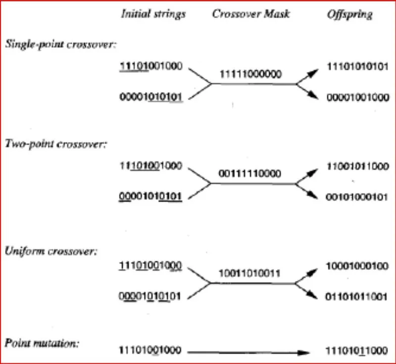
2) Determine fitness of population
3) Until convergence repeat:
a) Select parents from population b) Crossover and generate new population c) Perform mutation on new population.
"Convergence to the optimal point is the best foptimal value" whilst also reaching the performance quickly.
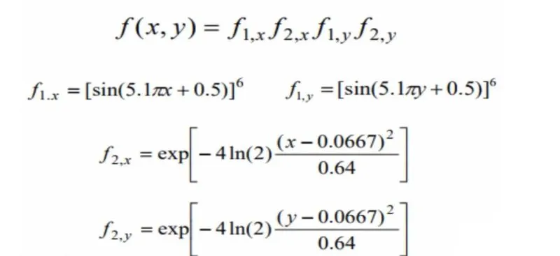
STALAGMITE :
clear all
close all
clc

%Defining our search space
x = linspace(0,0.6,180);
y = linspace(0,0.6,180);
num_cases  = 180;
%Creating a 2 Dimensional Array
[xx,yy] = meshgrid(x,y);

%Evaluating the stalagmite function
for i = 1:length(xx)
    for  j = 1:length(yy)
        input_vector(1) = xx(i,j);
        input_vector(2) = yy(i,j);
        f(i,j) = stalagmite1_func(input_vector);
    end
end


%Evaluating the stalagmite function
tic % Timer study Evaluation

for i = 1:num_cases
    [inputs , fopt(i)] = ga(@stalagmite1_func, 2);
    Xopt(i) = inputs(1);
    Yopt(i) = inputs(2);

end

fopt = -fopt;
study1_time = toc % Timer

figure(1)
subplot(2,1,1)
hold on
surfc(x,y,-f)
shading interp
plot3(Xopt,Yopt,fopt,'marker','o','markersize',5,'markerfacecolor','r')
title('Unbounded Inputs')
subplot(2,1,2)
plot(fopt)
xlabel('Iterations')
ylabel('Function Minimum')

%Evaluating the stalagmite function using the upper and lower bounds
tic % Timer study Evaluation

for i = 1:num_cases
    [inputs2 , fopt2(i)] = ga(@stalagmite1_func, 2,[],[],[],[],[0 0],[1 1]);%(fun,nvars,A,b,Aeq,beq,lb,ub)
    Xopt2(i) = inputs2(1);
    Yopt2(i) = inputs2(2);

end
fopt2 = -fopt2;
study2_time = toc % Timer

figure(2)
subplot(2,1,1)
hold on
surfc(x,y,-f)
shading interp
plot3(Xopt2,Yopt2,fopt2,'marker','o','markersize',5,'markerfacecolor','r')
title('Bounded Inputs')
subplot(2,1,2)
plot(fopt2)
xlabel('Iterations')
ylabel('Function Minimum')

%Evaluating the stalagmite function using the upper and lower bounds
options = optimoptions('ga','Populationsize',500)
tic % Timer study Evaluation

for i = 1:num_cases
    [inputs3 , fopt3(i)] = ga(@stalagmite1_func, 2,[],[],[],[],[0 0],[1 1],[],[],options); %(fun,nvars,A,b,Aeq,beq,lb,ub,lcon,nolcon,options)
    Xopt3(i) = inputs3(1);
    Yopt3(i) = inputs3(2);

end
fopt3 = -fopt3;
study3_time = toc % Timer

figure(3)
subplot(2,1,1)
hold on
surfc(x,y,-f)
shading interp
plot3(Xopt3,Yopt3,fopt3,'marker','o','markersize',5,'markerfacecolor','r')
title('Using Options Input')
subplot(2,1,2)
plot(fopt3)
xlabel('Iterations')
ylabel('Function Minimum')
function[results] = stalagmite1_func(input_vector)


x = input_vector(1);
y = input_vector(2);
f1_x = [sin(5.1*pi*x + 0.5)].^6;
f1_y = [sin(5.1*pi*y + 0.5)].^6;
t1 = (((x-0.0667).^2)/(0.64));
f2_x = exp(-4.*log(2)*t1);
t2 = (((y-0.0667).^2)/(0.64));
f2_y = exp(-4.*log(2)*t2);
results = -(f1_x*f1_y*f2_x*f2_y);
end
So
let's understand the matlab code,
- Primarily we initialise the values for x & y, which here is the search space parameter required to calculate the stalagmite function. we initialise it using the linspace command, from 0 to 0.6 for 180 values.
- We provide the num cases value similar to search space as we are going to use this part of the loop counter.
- We use the mesh gride command to convert the 1d array provided for x & y into 2d Array . There by we get a 180 X 180 Matrix for X & Y respectively.
- We use the for loop , i (rows) = 1 : length(xx) , & j(columns) = 1 : length(yy), and we assign a variable to every value from the corresponding matrix indexing that happens until the loop counter ends. Assigning xx & yy values to corresponding input vector(1) & input vector(2) respectively.
- Now we call the function , where we call the output arguments [ f(i,j) ] and also call the function handle stalagmite_func, inside which we give input vectors as input arguments. These are the values provided to the function code for matlab to calculate the foptimum value for each matrix index stored for 180 X 180 Matrix.
CASE : 1 - UNBOUNDED INPUTS
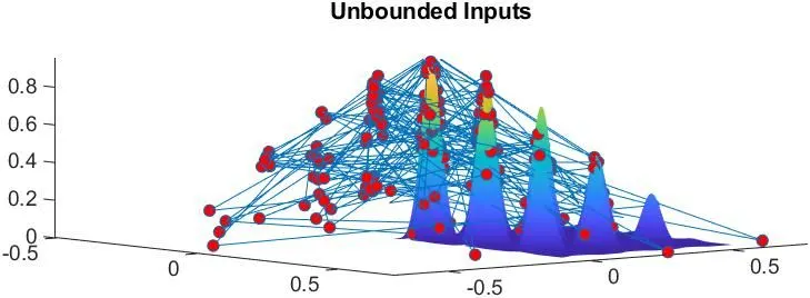
- Here we give output arguments, Inputs and Fopt(i) , we will be obtaining the coordinates x & y in the inputs and Optimum value which is the corresponding z value in fopt. So provide the variable xopt and yopt and assign the input vector values (1) & (2) to them respectively.
- And we call the genetic algorithm function to perform the calculation by providing the function template and also the set of variables inside the syntax.
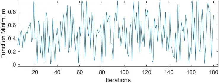
- As we obtain the values we surf plot our initial time space values, x & y values with -f value obtained. This is used under the subplot (2,1,1)
- Later, we call the hold on , and provide the respective coordinate values we obtain from genetic algorithm using a plot3 command for xopt , yopt & fopt.
- Here fopt = -fopt, is given because , we need our Z values to be plotted based on the stalagmite curve z's curve we passed part of the function code. If this wasn't provided, our points would get plotted below the surf plot, like the image provided below. Same also applies to the (x,y,-f).
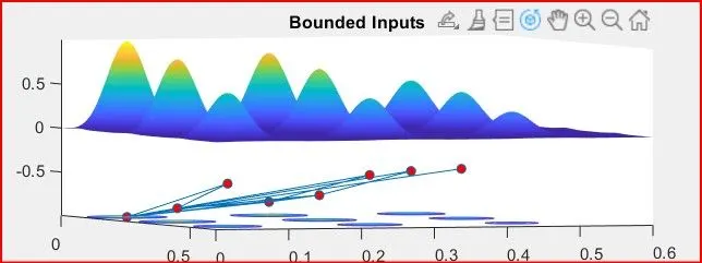
- We later provide the title name and marker size
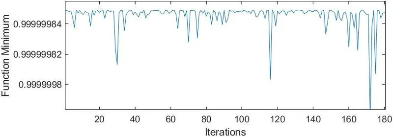
- We also do another subplot to infer the graph , from which we obtain the x & y values for each climb and descent
CASE 2 : BOUNDED INPUTS
- Here we give output arguments, Inputs and Fopt(i) , we will be obtaining the coordinates x & y in the inputs and Optimum value which is the corresponding z value in fopt. So provide the variable xopt and yopt and assign the input vector values (1) & (2) to them respectively.
- And we call the genetic algorithm function to perform the calculation by providing the function template and also the set of variables and providing the upper and lower limits part of the syntax.
- x = ga(fun,nvars,A,b,Aeq,beq,lb,ub) is the syntax.
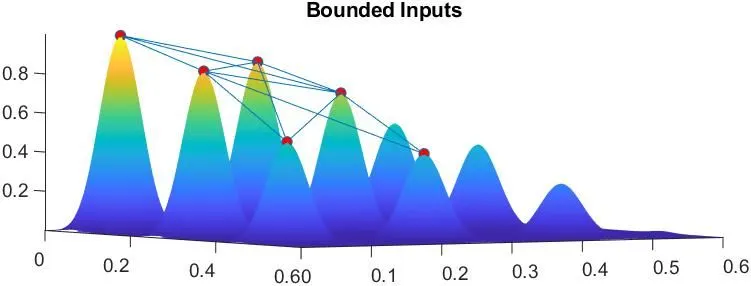
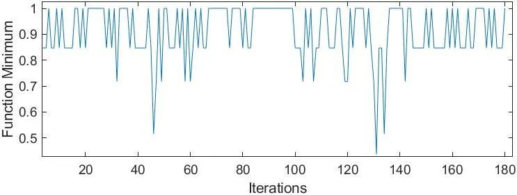
- As we obtain the values we surf plot our initial time space values, x & y values with -f value obtained. This is used under the subplot (2,1,1)
- Later, we call the hold on , and provide the respective coordinate values we obtain from genetic algorithm using a plot3 command for xopt , yopt & fopt.
- Here fopt = -fopt, is given because , we need our Z values to be plotted based on the stalagmite curve z's curve we passed part of the function code. If this wasn't provided, our points would get plotted below the surf plot, like the image provided below. Same also applies to the (x,y,-f).
- We later provide the title name and marker size
- We also do another subplot to infer the graph , from which we obtain the x & y values for each climb and descent
CASE 2 : OPTIONS INPUT
- Here we give output arguments, Inputs and Fopt(i) , we will be obtaining the coordinates x & y in the inputs and Optimum value which is the corresponding z value in fopt. So provide the variable xopt and yopt and assign the input vector values (1) & (2) to them respectively.
- And we call the genetic algorithm function to perform the calculation by providing the function template and also the set of variables and providing the upper and lower limits part of the syntax.
- x = ga(fun,nvars,A,b,Aeq,beq,lb,ub,nonlcon,intcon,options) is the syntax.
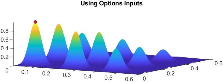
- As we obtain the values we surf plot our initial time space values, x & y values with -f value obtained. This is used under the subplot (2,1,1)
- Later, we call the hold on , and provide the respective coordinate values we obtain from genetic algorithm using a plot3 command for xopt , yopt & fopt.
- Here fopt = -fopt, is given because , we need our Z values to be plotted based on the stalagmite curve z's curve we passed part of the function code. If this wasn't provided, our points would get plotted below the surf plot, like the image provided below. Same also applies to the (x,y,-f).
- We later provide the title name and marker size
- We also do another subplot to infer the graph , from which we obtain the x & y values for each climb and descent
- "OPTIONS" - it is used to perform additional operations like increasing population size.
ERRORS :
- When calculating the stalagmite function, I initialised the value "stalagmite(input_vector1,input_vector2)" , later i realised , input vector is the variable name and we are just assigning xx & yy values to input vector position 1 (x) & position 2 (y).
- "results = (f1_x*f1_y*f2_x*f2_y);", i gave the final function formulae without a formulae, i corrected it with minus because, GA always calculates the minimum value. Inorder to find the maximum value, we insert the operator.
- Otherwise, i had minor typo issues.
EXPLANATION :
- We see that compared to first two studies, the last study consumed alot more time. This is because we've increased the number of iterations and population size. By which we have increased the number of times the code runs over a timespace.
- Speaking of timespace, whatever timespace we provide outside the function syntax, GA does not consider it.